The Normal Curve

1. The Normal Curve

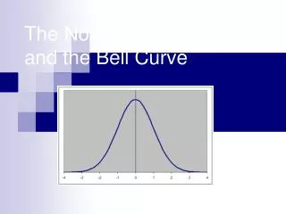
2. Introduction • The normal curve • Will need to understand it to understand inferential statistics • It is a theoretical model • Most actual distributions don’t look like this, but may be close • It is a frequency polygon that is perfectly symmetrical and smooth • It is bell-shaped and unimodal • Its tails extend infinitely in both directions and never intersect with the horizontal axis

3. Distances on The Normal Curve • Distances along the horizontal axis are divided into standard deviations and will always include the same proportion of the total area • This is true for a flat curve or a tall, narrow curve • It still divides into the same percentages • So, as the standard deviation of a normal distribution increases, the percentage of the area between plus and minus one standard deviation will stay the same

4. Distances from the Mean • Between plus and minus 1 standard deviations lies 68.26% of the area • Between plus and minus 2 standard deviations lies 95.44 % of the area • Between plus and minus 3 standard deviations lies 99.72 % of the area • On all normal curves, the area between the mean and plus one standard deviation will be 34.13%

5. Normally Distributed Variables • The normal curve will tell you what percentage of people are in any area of the curve • A normal distribution of 1,000 cases will have 683 people between plus and minus 1 standard deviation, about 954 people between plus and minus 2 standard deviations, and nearly all people (997) between plus or minus 3 standard deviations • Only 3 people will be outside 3 standard deviations from the mean, if the sample size is 1,000

6. Computing Z Scores • If your score on an exam was exactly 1 standard deviation above the mean, you would know that you did better than 84.13 percent of the students (the 50% below half, added to the 34.13% between half and the first standard deviation) • However, it’s not likely that your score will be the same as the mean plus exactly one standard deviation • So, Z scores are used to find the percentage of scores below yours from any place on the horizontal axis • The standardized normal distribution (or Z distribution) has a mean of 0 and a standard deviation of 1 • The curve becomes generic, or universal, and you can plug in any mean and standard deviation into it

7. Formula for Converting Raw Scores Into Z Scores • You plug your score into the X sub i position • You will be given the mean and the standard deviation of the sample

8. Calculating Z Scores • The Z score table gives the area between a Z score and the mean • For a Z score of -1.00, that area (in percentages) is 34.13% • If a Z score is 0, what would that tell you? • The value of the corresponding raw score would be the same as the mean of the empirical distribution

9. Using the Normal Curve to Estimate Probabilities • Can also think about the normal curve as a distribution of probabilities • Can estimate the probability that a case randomly picked from a normal distribution will fall in a particular area • To find a probability, a fraction needs to be used • The numerator will equal the number of events that would constitute a success • The denominator equals the total number of possible events where a success could occur

10. Example • The example in your book of your chances of drawing a king of hearts from a well-shuffled deck of cards • The fraction is 1/52 • Or can express the fraction as a proportion by dividing the numerator by the denominator • So 1/52 = .0192308 = .0192 • In the social sciences, probabilities are usually expressed as proportions • Or 1.92 percent of the time

11. Probabilities • Therefore, the areas in the normal curve table can also be thought of as probabilities that a randomly selected case will have a score in that area • So, the probability is very high that any case randomly selected from a normal distribution will have a score close in value to that of the mean • The normal curve shows that most cases are clustered around the mean, and they decline in frequency as you move farther away from the mean value

12. Probabilities • Can also say that the probability that a randomly selected case will have a score within plus or minus 1 standard deviations of the mean is 0.6826 • If we randomly select a number of cases from a normal distribution, we will most often select cases that have scores close to the mean—but rarely select cases that have scores far above or below the mean