Download
1 / 18
180 likes | 297 Views
REMOTE SENSING OF SOUTHERN OCEAN AIR-SEA CO 2 FLUXES. A.J. Vander Woude Pete Strutton and Burke Hales. Global CO 2 flux. Takahashi et al ., DSR I, 2009: 4.5 million data points. Takahashi et al ., DSR I, 2009: 3 million data points. Global CO 2 data coverage.

E N D
REMOTE SENSING OF SOUTHERN OCEAN AIR-SEA CO2FLUXES A.J. Vander Woude Pete Strutton and Burke Hales
Global CO2 flux Takahashi et al., DSR I, 2009: 4.5 million data points Takahashi et al., DSR I, 2009: 3 million data points
Southern Ocean & atmospheric CO2 Observations versus models Gruber et al. 2009
Why this may be better than observational methods? In some places there are no observations: pCO2from co-varying parameters is a way forward We can investigate smaller spatial scales: Limited by the resolution of the satellite data (kilometers), not sparse observations (~102 to 103 km) We can investigate seasonal and interannual variability: Links to long term changes in forcing: Southern Ocean winds
Steps to Create Predictive Satellite Algorithms: West Coast Example
Remote Sensing Climatology Monthly Data Sea Surface Height (cm) Chlorophyll a (mg/m3) Sea Surface Height: AVISO Multimission 1999-2008 Chlorophyll: SeaWiFS 1999-2002, MODIS/Aqua + SeaWiFS Merged 2003-2007, MODIS/Aqua 2007-2008 Wind speed: QuickSCAT 1999-2008 OI Reynolds SST: AVHRR 1999-2002, AVHRR+AMSR 2002-2008 Wind speed (m/s) OI Reynolds Sea Surface Temperature (°C)
Steps to Create Predictive Satellite Algorithms
Probablistic Self-Organizing Maps January March February region number There is some correspondence between SOM regions and the fronts Spatial and temporal coherence of the fronts from month to month Longhurst 1998
Overview of Predictive Satellite Algorithms Powell’s Optimization A Alkalinity and DIC from the McNeil climatologies Optimizing: Alk, DIC, Ti, Heating/Mixing term, Tcr Chlorophyll term Each has a constant, longitude, latitude & seasonal signal
pCO2 Results & Accuracy of Regional Model Spring Summer Region 4 May and June Predicted pCO2 (ppm) pCO2 (ppm) Red is a source to the atmosphere White is at atmospheric Blue is a sink, into the ocean Autumn Winter Observed Obo pCO2 (ppm) pCO2 (ppm)
Conclusions and future work Satellite algorithms offer a way to fill gaps and better quantify spatial and temporal variability of CO2 Next: -- Finishing the monthly algorithms, by region as well as Seasonal and interannual variability and produce maps of CO2 fluxes for the Southern Ocean -- More rigorous comparison with climatologies and models.
Thank you! • NASA for funding for this project • Maria Kavanaugh for her help with the PRSOM analysis and Ricardo Letelier’s lab use of their PRSOM/HAC code
CDIAC in situ pCO2 Coverage 1.4 million data points in the Southern Ocean, south of 40° S
SO GasEx observations and McNeil predictions
SO GasEx observations and Takahashi predictions
Southern Ocean & atmospheric CO2 Contemporary sink of: .1 to .5 PgC/yr (circulation models & atm and oceanic inversion models) .5 to .7 PgC/yr (pCO2 measurements, Takahashi et al. 2002) .15 to .65 PgC/yr (empirical estimated pCO2, McNeil et al., 2007) Gruber et al. 2009