Download
1 / 17
170 likes | 268 Views
Earth Observation for Agriculture – State of the Art –. F. Baret INRA-EMMAH Avignon, France. Outlook. The several needs for agriculture Observational Requirements Variables targeted / accessible Spatial Temporal Retrieval of key variables from S2 observations Generic algorithm

E N D
Earth Observation for Agriculture – State of the Art – F. Baret INRA-EMMAH Avignon, France
Outlook • The several needs for agriculture • Observational Requirements • Variables targeted / accessible • Spatial • Temporal • Retrieval of key variables from S2 observations • Generic algorithm • Specific algorithm • Assimilation • Conclusion/recommandations
The several needs for agriculture Precision agriculture Local Tools Pesticide Fertilizer Seeds Dealers Consultants Cooperatives Statistics Governments Control Traders Insurance Farmers Food Industry Food Industry Regional/International Governments
From observations to applications Assimilation of radiances Canopy Functioning Models Atmosphere Structure Biophysical variables estimates (Products) Assimilation of Products Biochemical content Soil • Need for biophysical products (LAI, fAPAR, fCover, Albedo) and their dynamics • Used as indicators for decision making • Input to crop process models • Smooth expected temporal course (allows smoothing / real time estimates) • Allows validation • Provide uncertainties • Need for crop classification
Observational requirements: Variables targetted (and accessible!) • Biophysical variables of interest: • LAI (actually GAI) • Green fraction (FAPAR, FCOVER) • Chlorophyll content • Water content • Soil related characteristics • Crop residue estimates
Spectral requirements Correction for the atmosphere Sampling the absorption of main leaf constituants
Observationalrequirements: Spatial resolution Variabilitywithin pixel Number of patches/pixel Purity of pixel Large differences between 10-20-60 m with 100-250-1000m • Precision agriculture: intra-field variability • Other applications: • Fields • Species (regional assessment of production)
Observationalrequirements: Revisitfrequency • Getting information every 100°C.day: • One month in winter • 5 days in summer Green Fraction Green Fraction Accounting for clouds (≈50% occurence) Providing information on crop state at specific stages (± 1 week) Monitoring crops for resources management
Retrieval of key variables from S2: Genericalgorithms Applicable everywhere with variable accuracy but good consistency Allows continuity with hectometric/kilometric observations Based on simple assumptions on canopy structure
Retrieval of key variables from S2: Genericalgorithmsapplied to severalsensors Landsat IRS DMC Rapideye SPOT4 Landsat SPOT4 SPOT4 SPOT4 Time Grassland_1 Grassland_2 Shrubland Forest (oak) Capacity to build a consistent time series from multiple sensors Virtual constellation Possible spectral sensitivity residual effects
Retrieval of key variables from S2: Specificalgorithms • Need knowledge of land-use (species / cultivars) • On the fly land-use (continuously updated) • Allows using prior distribution of canopy characteristics • Canopy Structure • Leaf properties (structure, chlorophyll, SLA, water, surface effects …) • Need calibration over • detailed radiative transfer model • Comprehensive experiments
Calibration over radiative transfermodels Generic (Turbid) Specific (3D) Maize Estimated LAI Estimated LAI Measured LAI Measured LAI Vineyard Estimated LAI Estimated LAI Measured LAI Measured LAI Better use more realistic 3D model than turbid medium (generic) model From Lopez-Lozano, 2007
Calibration over experiments Green Fraction Use of (HT) phenotyping / agronomical Experiments Characterize specific structural traits
Combinationwithcropmodels Ancillary Information/data ? Process model (dynamic) Radiative Transfer Model Diagnostic variables Variables of interest Radiance observations Model Parameters Assimilation allows to: • input additional information in the system: • Knowledge on some processes • Exploitation of ancillary data (climate, soil, …) • exploit the temporal dimension: process model as a link between dates • access specific processes / outputs (biomass, yield, nitrogen balance) • Run process models in prognostic mode : simulations for other conditions
CombinationwithcropmodelsExample of assimilation Question: How to optimize the nitrogen amount for a field crop ? • Inputs: • Climate (past) • Soil (Prior knowledge of characteristics, but no spatial variability) • Technical practices (sowing date, …) • Crop model (STICS) and some crop parameters • 3 flights with CASI instrument • Outputs: • Map of nitrogen content (QN)
Assimilation of (RS) observations Prior distribution of inputs 200 000 cas Prior QN (kg/ha) Climate past' Flight 3 Crop model Flight 2 Soil Flight 1 Cultural Pract. Actual QN (kg/ha) Prior distribution of outputs LAI, Cab Cost function Remote sensing Estimates LAI, Cab Posterior QN (kg/ha) Flight 3 Flight 2 Posterior distribution of inputs 1 000 cases Flight 1 Actual QN (kg/ha)
Conclusion & Recommandations • S2 very well adapted to requirements for agriculture • Following issues to be solved: • Organize the validation / calibration to capitalize on the work done • Build an archive (anomalies) • Fusion with other missions for improved revisit frequency at the level of biophysical variables (or higher) products • decametric missions (Rapid-eye, DMC, Venµs, , SPOT6/7, LDCM…) • hectometric resolution observations (PROBA-V, S3 …) • Development of algorithms for: • Top of canopy fused products at 10 m resolution and original resolutions • on the fly classification (continuously updated) • specific products per crop/cultivar • Patch (object) oriented algorithm to take into account • the continuity within patches • The variability within patches (texture) • Development of combination of S2 data with crop models (Assimilation) • Improved description of canopy structure by models in relation to function • Simplification of crop models (meta-model)