Download
1 / 30
300 likes | 443 Views
Polymorphism & Variant Analysis Lab. Saurabh Sinha. Powerpoint by Casey Hanson. Exercise. In this exercise, we will do the following: . Gain familiarity with a graphical user interface to PLINK

E N D
Polymorphism &Variant Analysis Lab Saurabh Sinha Powerpointby Casey Hanson Polymorphism and Variant Analysis Lab v1 | Saurabh Sinha
Exercise In this exercise, we will do the following:. • Gain familiarity with a graphical user interface to PLINK • Run a Quality Control (QC) analysis on genotype data of 90 individuals of two ethnic groups(Hong Chinese and Japanese) genotyped for ~230,000 SNPs. • Use our QC data to perform a genome wide association test (GWAS) across two phenotypes: case and control. We will compare the results of our GWAS with and without multiple hypothesis correction. Polymorphism and Variant Analysis Lab v1 | Saurabh Sinha
Step 0A: Shared Desktop Directory For viewing and manipulating files on the classroom computers, we provide a shared directory in the following folderon the desktop: classes/mayo In today’s lab, we will be using the following folder in the shared directory: classes/mayo/sinha2 Polymorphism and Variant Analysis Lab v1 | Saurabh Sinha
Step 0B: Copying GWAS Directory to Desktop Navigate to our shared folder directory: classes/mayo/sinha2/ Right click on the gwas folder and select Copy. Right click on the Desktop and select Paste. Polymorphism and Variant Analysis Lab v1 | Saurabh Sinha
Dataset Characteristics Polymorphism and Variant Analysis Lab v1 | Saurabh Sinha
The PED File Format The PED File Format specifies for each individual their genotype for each SNP and their phenotype. Family ID is either CH (Chinese) or JP (Japenese) Paternal and Maternal IDs of 0 indicate missing. Sex is either Male=1, Female=2, Other=Unknown Phenotype is either 0 = missing, 1 = affected, 2 = unaffected. Polymorphism and Variant Analysis Lab v1 | Saurabh Sinha
The MAP File Format The MAP File Format specifies the location of each SNP. Note: Morgans (M) are a special kind of genetic distance derived from chromosomal recombination studies. Morganscan be used to reconstruct chromosomal maps. Polymorphism and Variant Analysis Lab v1 | Saurabh Sinha
Configuring gPLINK In this exercise, we will configure gPLINK to work with our data. Additionally, we will perform a format conversion to speed up our QC analysis. Finally, we will validate our conversion and see what individuals and SNPs would be filtered out with default filters for QC analysis. Polymorphism and Variant Analysis Lab v1 | Saurabh Sinha
Step 1: Starting gPLINK gPLINK is a graphical user interface, written in JAVA, to the command line program PLINK. To start gPLINK, navigate to the gwasdirectory we copied to the Desktop. Double click on gplink.jar. A window should appear similar to the one on the right. Polymorphism and Variant Analysis Lab v1 | Saurabh Sinha
Step 2A: Configuring gPLINK Click on the Project item on the Menu Bar. Select Open from the drop down menu. The pop-up window should look similar to the screenshot below. Click on Browse. Polymorphism and Variant Analysis Lab v1 | Saurabh Sinha
Step 2B: Configuring gPLINK In the file browser, navigate to the Desktop. Click on the gwas directory and click Open. Click OK on the OpenProject window. Polymorphism and Variant Analysis Lab v1 | Saurabh Sinha
Step 2C: Configuring gPLINK You should see the files in the gwas folder in the Folder Viewer on the left hand side of gPLINK. Polymorphism and Variant Analysis Lab v1 | Saurabh Sinha
Step 3A: Creating a Binary Input File Click the PLINK item on the Menu Bar. Click Data Management. Click Generate fileset. In the next window, select Standard Input on the tab bar. Select wgas1 under Quick Fileset. Check Binary fileset. Under Output File input wgas2. Click OK. Polymorphism and Variant Analysis Lab v1 | Saurabh Sinha
Step 3B: Creating a Binary Input File On the Execute Command window, click OK. This will convert our wgas1files to a binary format. Under the Operations Viewer, you will wgas2 with an R next to it indicating running. Wait for it to turn GREEN. Polymorphism and Variant Analysis Lab v1 | Saurabh Sinha
Step 3C: Creating a Binary Input File In the Folder Viewer, you should see a bunch of new wgas2 files created during the file creation process. Polymorphism and Variant Analysis Lab v1 | Saurabh Sinha
Step 4A: Validating the Conversion Click the PLINK item on the Menu Bar. Click Summary Statistics. Click Validate Fileset. In the next window, select Binary Input on the tab bar. Select wgas2 under Quick Fileset. Under Output File input validate. Click OK. Polymorphism and Variant Analysis Lab v1 | Saurabh Sinha
Step 4B: Validating the Conversion On the Execute Command window click OK. Wait for the command to finish (validate will show the icon) Click on the validate track: Polymorphism and Variant Analysis Lab v1 | Saurabh Sinha
Step 4C: Validating the Conversion Look in the Log viewer 46834 out of ~ 230,000 SNPs were removed because the failed the MAF. 623 SNPS were removed because they were not genotyped in enough individuals (minimum, 90%). Polymorphism and Variant Analysis Lab v1 | Saurabh Sinha
Step 4D: Validating the Conversion Click the + adjacent to the Validate track to expand it. Click the + adjacent to the Output track to expand it. Right click validate.irem and click Open in default viewer. You should see the following: JA19012 NA19012 The family ID is JA19012 (Japanese) and the individual ID is NA19012. This individual was removed because of a low genotyping rate. Polymorphism and Variant Analysis Lab v1 | Saurabh Sinha
Quality Control Analysis In this exercise, we will perform Quality Control Analysis (QC) to filter our data according to a set of criteria. Polymorphism and Variant Analysis Lab v1 | Saurabh Sinha
Quality Control Filters The validation tool will impose the following criterion on our data. Polymorphism and Variant Analysis Lab v1 | Saurabh Sinha
Step 5A: Quality Control Analysis Click the PLINK item on the Menu Bar. Click Data Management. Click Generate Fileset. In the next window, select Binary Input on the tab bar. Select wgas2 under Quick Fileset. Click Binary fileset. Under Output File input wgas3. Click Threshold. Polymorphism and Variant Analysis Lab v1 | Saurabh Sinha
Step 5B: Quality Control Analysis On the Threshold window: Set Minor allele frequency to 0.01. Set Maximum SNP missingness rate to 0.05. Set Maximum individual missingness rate to 0.05 Set Hardy Weinberg equilibrium to 0.001 Click OK. Polymorphism and Variant Analysis Lab v1 | Saurabh Sinha
Step 5C: Quality Control Analysis Click OK. On the Execute Command window, click OK. This will create a new set of files prefixed gwas3 that are filtered according to the thresholds on the previous slide. Polymorphism and Variant Analysis Lab v1 | Saurabh Sinha
Genome Wide Association Test (GWAS) In this exercise, we will a GWAS on our filtered data across two phenotypes: a case study and control. We will then compare the results between unadjusted p-values and multiple hypothesis corrected p-values. Polymorphism and Variant Analysis Lab v1 | Saurabh Sinha
Step 6A: GWAS Click the PLINK item on the Menu Bar. Click Association. Click Allelic Association Tests. In the next window, select Binary Input on the tab bar. Select wgas3 under Quick Fileset. Click Adjusted p-values. Under Output File input assoc1. Click OK. Polymorphism and Variant Analysis Lab v1 | Saurabh Sinha
Step 6B: GWAS On the Execute Command window, click OK. This will perform the GWAS analysis on our data and store the results under assoc1 in the main window of gPLINK. Polymorphism and Variant Analysis Lab v1 | Saurabh Sinha
Step 7: GWAS Without Multiple Hypothesis Correction The SNP values from our GWAS with no multiple hypothesis correction are located in the 9th column of assoc1.assoc. You can inspect this file by Right Clicking it and selecting Open in default viewer. Open in Excel if you want to sort by p-value. Overall, 13,238 SNPS survive at value of 0.05 WITHOUT Multiple Hypothesis Correction. The top 5 are shown below, after using the unixsort, awk, and head commands. Polymorphism and Variant Analysis Lab v1 | Saurabh Sinha
Step 8: GWAS With Multiple Hypothesis Correction The SNP values from our GWAS with multiple hypothesis correction are located in the 9th column of assoc1.assoc.adjusted. You can inspect this file by Right Clicking it and selecting Open in default viewer. Overall, only 4 SNPS!!! show a Bonfferoni Correction of less than 1. Polymorphism and Variant Analysis Lab v1 | Saurabh Sinha
Step 9: P-Value Distribution Graph This plot requires Haploview which we will not go into configuring at the present moment. It is possible to graph the negative log of our p-value, , for all SNPS to give a pictoral view of the distribution of p-values. Note, this is conducted for uncorrected p-values. Polymorphism and Variant Analysis Lab v1 | Saurabh Sinha