Download
1 / 30
340 likes | 991 Views
Design of Experiments. 2 k Designs. Catapult Experiment.

E N D
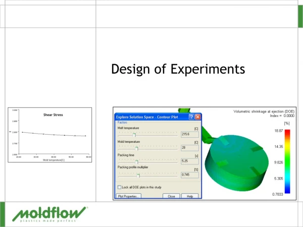
Design of Experiments 2k Designs
Catapult Experiment An engineering statistics class ran a catapult experiment to develop a prediction equation for how far a catapult can throw a plastic ball. The class manipulated two factors: how far back the operator draws the arm (angle), measured in degrees, and the height of the pin that supports the rubber band, measured in equally spaced locations. The results follow… L. Wang, Department of Statistics University of South Carolina; Slide 2
Catapult Experiment L. Wang, Department of Statistics University of South Carolina; Slide 3
This is a 22 (levelfactor) Design Height (-1,1) (1,1) Angle (1,-1) (-1,-1) L. Wang, Department of Statistics University of South Carolina; Slide 4
Response Notation • a = Average of responses when A (Angle) is high and B (Height) is low. • b = Average of responses when B (Height) is high and A (Angle) is low. • ab = average of responses when both A (Angle) and B (Height) are high. • (1) = Average of responses when both A (Angle) and B (Height) are low. L. Wang, Department of Statistics University of South Carolina; Slide 5
This is a 22 (levelfactor) Design b ab Height (-1,1) (1,1) Angle (1,-1) (-1,-1) a (1) L. Wang, Department of Statistics University of South Carolina; Slide 6
Catapult Experiment L. Wang, Department of Statistics University of South Carolina; Slide 7
Catapult Experiment – Main Effects Effect of Angle = avg response at high level – avg response at low level L. Wang, Department of Statistics University of South Carolina; Slide 8
Catapult Experiment – Main Effects Effect of Height = avg response at high level – avg response at low level L. Wang, Department of Statistics University of South Carolina; Slide 9
Interactions • If Angle and Height interact, then the effect of Angle depends on the specific level of Height. • An interaction plot plots the means of one factor given the levels of the other factor. L. Wang, Department of Statistics University of South Carolina; Slide 10
Interaction Plot ab A v g D i s t 2 b a Height(-1): 2 1 (1) Angle 140 180 L. Wang, Department of Statistics University of South Carolina; Slide 11
Interaction of A (Angle) and B (Height) We have a positive interaction which is smaller in size than the main effects (effect of Angle = 65 and effect of Height = 55.5. L. Wang, Department of Statistics University of South Carolina; Slide 12
The model we are fitting is yi is the distance for the ith test run β0 is the y-intercept β1 is the regression coefficient associated with angle β2 is the regression coefficient associated with height β12 is the regression coefficient associated with angle/height interaction εi is the random error L. Wang, Department of Statistics University of South Carolina; Slide 13
Table of Contrasts This table tells us how to combine the average response for each treatment combination to form the numerator of our estimate of the effect. For two-level factorial designs, the denominator for estimating main effects and interactions will always by one-half of the number of distinct factorial treatment combinations. Ex: 22 = 4, so our denominator is 2. Use total number of distinct treatment combinations as denominator for the intercept. L. Wang, Department of Statistics University of South Carolina; Slide 14
Model Coefficients are Slopes • A slope represents the expected change in the response when we increase one factor by one unit while holding the other factor constant. • Going from -1 to 1 in a factor represents movement of two units. • So: L. Wang, Department of Statistics University of South Carolina; Slide 15
Multiple Linear Regression • Dependent Variable: Distance • Independent Variables: Angle, Height, Angle*Height • Parameter estimates: • ANOVA table: L. Wang, Department of Statistics University of South Carolina; Slide 16
2k Full Factorial Designs • We will look at every possible combination of the two levels for k factors. • Let’s extend our catapult Experiment to include: • Angle: 180, Full • Peg Height: 3, 4 • Stop Position: 3, 5 • Hook Position: 3, 5 • Each combination was run twice. L. Wang, Department of Statistics University of South Carolina; Slide 17
L. Wang, Department of Statistics University of South Carolina; Slide 18
L. Wang, Department of Statistics University of South Carolina; Slide 19
24 Model: L. Wang, Department of Statistics University of South Carolina; Slide 20
Effects • Use Contrast Table for numerator. • Denominator is one half the number of distinct combinations. • Use total number of distinct combinations as denominator for Intercept. L. Wang, Department of Statistics University of South Carolina; Slide 21
L. Wang, Department of Statistics University of South Carolina; Slide 22
Fractions of 2k Factorial Designs • Used to reduce the total number of treatment combinations while preserving the basic factorial structure. • Main effects tend to dominate two-factor interactions, two-factor interactions tend to dominate three-factor interactions, and so on. • We will sacrifice the ability to estimate the higher-order interactions in order to reduce the number of treatment combinations. L. Wang, Department of Statistics University of South Carolina; Slide 23
Half Fraction of 23 Design L. Wang, Department of Statistics University of South Carolina; Slide 24
Half Fraction of 23 Design L. Wang, Department of Statistics University of South Carolina; Slide 25
Aliasing Effects • When we alias one effect with another (eg: Aliasing effect of A with effect of BC), we can not distinguish one effect from the other (eg: we can not distinguish effect of A from effect of BC.). • Positive half fraction of a 23 design uses x1x2x3 = 1 to select the treatment combinations to be run. • Negative half fraction of a 23 design uses x1x2x3 = -1 to select the treatment combinations to be run. L. Wang, Department of Statistics University of South Carolina; Slide 26
Aliasing Effects • We say that ABC is the defining interaction. • General notation: 23-1 • 2 indicates number of factor levels. • Exponent 3 indicates the number of factors. • Exponent -1 indicates a half (2-1) fraction. • Total number of treatment combination is 23-1 = 4. L. Wang, Department of Statistics University of South Carolina; Slide 27
The Alias Structure • ABC as the defining interaction is equated to the intercept, I. • Then add each effect to the defining interaction using modulo 2 arithmetic. • Eg: A + ABC = BC B + ABC = AC C + ABC = AB L. Wang, Department of Statistics University of South Carolina; Slide 28
The Alias Structure or L. Wang, Department of Statistics University of South Carolina; Slide 29
Warning • Remember that aliases can not be distinguished from one another, so be careful what you alias. L. Wang, Department of Statistics University of South Carolina; Slide 30