Download
1 / 65
680 likes | 1.07k Views
RISK ASSESSMENT. Emissions. Transport and Fate. Concentrations. Exposure. Dose. Dose-response Relationship. Health Risk. Schematic overview of a Health Risk Assessment. THEME 2 TRANSPORT AND FATE. ENVIRONMENTAL EMISSIONS Air Stack emissions, incineration, manufacturing..

E N D
Emissions Transport and Fate Concentrations Exposure Dose Dose-response Relationship Health Risk Schematic overview of a Health Risk Assessment
THEME 2 TRANSPORT AND FATE
ENVIRONMENTAL EMISSIONS • Air • Stack emissions, incineration, manufacturing.. • Fugitive emissions (tanks of storage, leakage, waste storage) • Losses during use and transport • Water • Effluents treatment in production. • Spilling during production and distribution • Losses during transport • Storage after use • Soil • Controlled and uncontrolled spill. • Losses during use
TRANSPORT OF CONTAMINANTS IN AIR • Gaussian plume shape (H – mixing layer height, h – stack height, H – plume height assuming flat terrain, H* - plume height above terrain)
TRANSPORT IN AIR Air dispersion models: Gaussian plume model. where: c(x,y,z) = concentration of pollutant at receptor location (x,y,z) Q = pollutant emission rate (mass per unit time) u = mean wind speed at release height y =standard deviation of lateral concentration distribution at downwind distance z =standard deviation of vertical concentration distribution at downwind distance x h = plume height above terrain
DATA INFORMATION • Stack Information: • Location • Diameter of the stack • High • Flow Emissions • Gas Emission Temperaure • Gas speed • Concentrations of the contaminants
Cartographic dates • Institut Cartogràfic de Catalunya (http://www.icc.es/downlod) • Buildings • Meteorological dates: • (Generalitat de Catalunya: http://www.gencat.es) • (Instituto Nacional de Meteorología: //www.inm.es) • (Ministerio de Medio Ambiente: //www.mma.es) • Wind speed and direction • Rainfall • Sum radiation • Air Estability
Elevation of the area (data from MiraMon/ Generalitat de Catalunya)
Pollution Transport Isopleth lines obtained from the Gaussian model (Industrial Source Complex, ISC 3) Particulate matter Gas phase Principal wind directions to: ENE (19.0 % ) NE (18.5 %).
Air dispersion models • USEPA • (http://www.epa.gov/scram001/tt22.htm) • ISC3 • (http://www.air-dispersion-model.com/html/air-quality-des.html) • CALPUFF • (http://www.src.com/balpuff/calpuff3.htm)
WATER DISPERSION MODEL GREAT-ER Geography-referenced Regional Exposure Assessment Tool for European Rivers. Waste water pathway of “down the drain” chemicals [Boeije (1999)]
A GREAT-ER screenshot, showing the Rur catchment. The river network and the cities in the densly populated area can be seen.
FATE AND TRANSPORT IN SOIL MODFLOW
DARCYS’S LAW dh Q = KA dL Q= Flow rate K = Hydraulic conductivity or coefficient of permeability (m/day) A= Sectional area dh/dL= Hydraulic gradient FLOW VELOCITY Q KA(dh/dL) dh v = = = K A A dL
FATE AND TRANSPORT PRROCESSES • ADVENTION • DISPERSION • CHEMICAL PROCESSES • Precipitation/solution • Ionic Interchange • Redox processes • PHYSIS PROCESSES • Adsortion • Volatilization • BIOLOGICAL PROCESSES
SUMMARY Key factors controlling environmental fate 1.- The prevailing environmental conditions 2.- Physical-chemicalsproperties 3.-The patterns of use
MULTI-COMPARTMENT ENVIRONMENTAL SYSTEM PARTITION MODELS These models describe the partition of the contaminant between various compartments
CHEMODYNAMICS • Chemicals differ so greatly in their behavior. • Chloroform, evaporate rapidly and are dissipated in the atmosphere. • DDT, partition into the organic matter of soils and sediments and the lipids of fish, birds and mammals. • Phenols and carboxylic acids tend to remain in water where they may be subject to fairly rapid transformation processes such as hydrolysis, biodegradation and photolysis.
PHYSICO-CHEMICAL PROPERTIES • The key properties are: • Solubility in water (Ks) • Vapor pressure (P) • Henry's Law Constant (H) • Octanol-water partition coefficient (Kow) • Air-water partition coefficient (Kaw) • Dissociation constant in water • Susceptibility to degrading • Transformation reactions. • Other essential molecular descriptors are: • Molecular mass (MW) • Molar volume (MV)
Quantitative Structure-Property Relationships (QSPRs) The ultimate goal is to use information about chemical structure to deduce physical-chemical properties, environmental partitioning and reaction tendencies, and even uptake and effects on biota.
Air-Water partitioning • Solubility in water and Vapor pressure are both "saturation" properties, i.e., they are measurements of the maximum capacity which a phase has for dissolved chemical. • Water Solubility • Is the concentration of a compound that is in equilibrium in a saturated solution at a given temperature. • Water Solubility ranges • Low solubility: < 10 ppm (mg/L) • Medium Solubility : 10 - 1000 ppm • High solubility > 1000 ppm
Air-Water partitioning • Vapor pressure P (Pa) • Can be viewed as a "solubility in air” (mol/m3) • Is an indicator of the ability of a chemical to volatile. • Pa = P/RT ; R= 8.314 Pa m3 /mol·K • T = ºK • Low Vp: <1.0 E-06 mm Hg • Medium Vp: 1.0 E-06 - 1.0 E-02 mm Hg • High Vp > 1.0 E-02 mm Hg
Air-Water partitioning • Henry’s law constant (H) : • Is a partition coefficient that expresses the ratio of the • chemical’s concentrations in air and water at equilibrium • and is used as an indicator of a chemical’s potential to • volatilize. • Henry's law constants can be calculated from the ratio of vapor pressure and aqueous solubility (H = Vp/ S ) • Vapor pressure and solubility thus provide estimates of air-water partition coefficients K or Henry's law constants H(Pa·m3 /mol), and thus the relative air-water partitioning tendency.
Soil-Air partitioning • Koa. Octanol-air Partition coefficient • Characterize the partitioning of organic chemicals between the atmosphere and soil or foliage
Organic-Water partitioning • Octanol-Water Partition Coefficient (Kow): • Equilibrium ratio of the concentrations of a chemical in n-octanol • and water, in dilute solution. • KOW = CO/CW • CO= concentration in octanol phase • CW = concentration in water phase • Provides a direct estimate of hydrophobicity or of partitioning O-W tendency from water to organic media such as lipids, waxes and natural organic matter such as humin or humic acid.
Organic-Water partitioning • Kow ranges: • Low Kow <500 • Medium Kow : 500 - 1000 • High Kow > 1000
Organic carbon partition coefficient (Koc) • Ratio of the amount of a chemical adsorbed per unit weight of • organic carbon in the soil or sediment to the concentration of the • chemical in solution at equilibrium. • mg adsorbed chemical / kg organic carbon • Koc = • mg of dissolved chemical /L of solution • Koc = foc * 0.48 Kow • Koc and the Kow indicates the chemical’s potential to bind to organic • carbon in soil and sediment. • The Koc and the Kow is used also to estimate the potential for an • organic chemical to move from water into lipid and has been • correlated with bioconcentration in aquatic organisms. Organic-Water partitioning
Organic-Water partitioning • Koc values: • Koc <1000 will no be adsorbed to soil 0ºC • Koc =1000 –10 000 could behave either way • Koc >10 000 will adsorbed to soil
Soil-Water partitioning • Adsorption Ratio (Kd): • Amount of a chemical adsorbed by a sediment or soil (i.e., the solid phase) divided by the amount of chemical in the solution phase which is in equilibrium with the solid phase, at a fixed solid/solution ratio. • It is generally expressed in micrograms of chemicalsorbed per gram of soil or sediment.
Water-fish partitioning Bioconcentration Factors (BCF) The quotient of the concentration of a chemical in aquatic organisms at a specific time or during a discrete time period of exposure divided bythe concentration in the surrounding water at the same time or during the same period. BCF (Kb) = 0.05 K OW 0.05 corresponds to a 5% lipid content of the fish Kb , the organic carbon-water partition coefficient Sorption Coefficients:
DEGRADATIONS FACTORS • HALF-LIVE • Time that it takes for the chemical to be reduced by one-half of its original amount • Depending factors: • Sunlight intensity (photolitic half-life) • Hydroxyl radical concentration • The nature of the microbial community • Temperature
Thermodynamic Relationships • Fugacity “f” • Represents the partial pressure of chemical in a particular • medium and controls the movement of chemical between media. • Represent the “escaping tendency” and is identical to the partial pressure of ideal gases. • Fugacity (f) : (Pa) or (at)f= c/Z • c = concentration in the considered phase (mol/ m3) • Z= fugacity capacity (mol/m3 Pa) or mol/l at • Zw =1/H • By equilibrium between two phases f=0
Applying the equation for ideal gases p V = R n T c = p/RT = f/(RT) Comparing with f= c/Z The fugacity capacity in airZa Za = 1/RT At equilibrium between water and air, the fugacity is the same in the two phases ca Za = cw Zw ca /cw = Zw /Za = Kaw Simirlaly between water and soil cs /cw = Zw /Zs = Ksw
FUGACITY CAPACITY Zair = 1/RT (mol/m3 Pa) Z water = 1/H (mol/m3 Pa) Z soil = foc * Kow/H (mol/m3 Pa) Partition coeficients : ZAW = ZA/ZW (Air-water partition Coeficient) ZAS = ZA/Zs (Air-soil partition Coeficient) ZWsed = Zw/Zsed (water-sed partition Coeficient) ZwS = Zw/Zs (water-soil partition Coeficient)
Example A chemical has a MW of 200 g/mol and a water solubility of 20 mg/l, which gives a vapor pressure of 1 Pa. The distribution coefficient octanol-water is 10,000 and Koc = 4000. How will an emission of 1000 moles be distributed in a region with an atmosphere of 6 x 10 8 m3, a hydrosphere of 6x10⁶ m3, a lithosphere of 50,000 m3 with a specific gravity of 1.5 kg/l and an organic carbon content of 10%. Biota fish is estimated to be 10 m3 , specific gravity 1.00 kg/l and a lipid content of 5%. The temperature is 20ºC.
Fugacities capacities: Za = 1/RT mol/m3 Pa Zw = 1/H = S/Pv moles /m3 Pa Zs = foc * Kow/H = foc Koc moles/m3 Pa Zbiota = foc * Kow moles/m3 Pa ZiVi = mol/Pa f= Total mol /ZiVi = Pa Concentrations: ca = fZa moles/m3 cw = f Zw moles/m3 cs = f Zs moles/m3 cbiota = f Zbiota moles/m3 = mols emission
Solution Fugacities capacities: Za = 1/RT = 1/8.314 *293 = 0.00041 mol/m3 Pa Zw = (20/200)/1 = 0.1 moles /m3 Pa Zs = 0.1 x 0.1x 4000 = 40 moles/m3 Pa Zbiota = 0.1 x 0.05x10,000 = 50 moles/m3 Pa ZiVi = 0.00041x6x108 + 0.1 x 6x106 + 40 x 50000+ 10x 50 = = 2846500 mol/Pa f= M/ZiVi = 1000 moles /2846500 mol/Pa = 3.51 x 10⁻⁴ Pa Concentrations: ca = fZa = 3.51 x 10-4x 0.00041 = 1.44 x 10⁻⁷moles/m3 cw = f Zw = 3.51 x 10-4 x 0.1 = 3.51 x 10⁻⁵ moles/m3 cs = f Zs = 3.51 x 10-4 x 40 = 1.404 x 10⁻² moles/m3 cbiota = f Zbiota = 3.51 x 10-4 x 50 = 1.755 x 10⁻² moles/m3 = 999.2 moles ~ 100 mols emission
FATE AND TRANSPORT How is a chemical moved in the environment by natural means? • AIR ENVIRONMENT • Photodegradate • Be inhaled • Be absorbed • Fallout in non-contaminate environment
SOIL COMPARTMENT • Leach through the soil • Run off the soil • Adsorb in the soil • Biodegradate in soil • Accumulate in the soil • Bioaccumulate in plants and animals or be metabolized • Be phototransformer • Contaminate aquatic environment
AQUATIC ENVIRONMENT • Biodegradate • Photodegradate • Bioaccumulate in aquatic organism • Volatilize • Contaminate plants, animals and well water • Adsorb to suspended and bottom sediment
PLANTS COMPARTMENT • Be metabolized • Bioaccumulate • Be eaten by humans and other animals