Download
1 / 18
180 likes | 356 Views
Unsolved Problems on Noise 2008 Lion, June 3 rd. Crackling Noise and Universality in Fracture Systems Gianni Niccolini and Gianfranco Durin Istituto Nazionale di Ricerca Metrologica; Torino, Italy. Crackling Noise = the system response to continuously changing external

E N D
Unsolved Problems on Noise 2008 Lion, June 3rd • Crackling Noise and Universality in Fracture Systems • Gianni Niccolini and Gianfranco Durin • Istituto Nazionale di Ricerca Metrologica; Torino, Italy
Crackling Noise = the system response to continuously changing external conditions through discrete, impulsive events. Event sizes span a broad range of scales following regular behaviour (i.e., power-law) • Many physical systems crackle (fracture systems); two examples: • The earth responds to the slow strains imposed by continental drift with violent and intermittent earthquakes. • A concrete specimen emits intermittent and sharp acoustic emissions (AEs) as it is slowly loaded.
The Earth crackles typical time history of earthquakes in a spatial region and a time period The Gutenberg-Richter (GR) law: N(M≥ Mth)10 –bMth Magnitude with logarithmof event size: M LogS →N(S≥ Sth) Sth–b
The range of this law extends from lab scale unnoticeable trembles (i.e., the acoustic emissions ) to catastrophic earthquakes: universality ( the same behaviour on a wide range of scales) Crackling noise is defined only by the size response of the system There is any reference to its time evolution We analyze time properties of fracture systems in order to investigate universal features of fracture phenomena
Earthquakes and AEs point events in space, time and magnitude • Hypocentres coordinates • Initiation time ti • Size magnitude Mi • Drastic (but useful) simplification • Later on the spatial degrees of freedom will be disregarded
Consider a fixed region and a fixed time window T (space-time window w) • Consider events with magnitude larger than a threshold Mth • Compute waiting times as the time between consecutive events: • τi ≡ ti–ti–1 • (Bak et al., 2002; Corral, 2004) Broad scale of times (from seconds to years) GR rate (Number of earthquakes per Unit time in w) very poor temporal Description: R(Mth) = N(Mth) / T=< τ (Mth)>–1
We consider distributions of waiting times: D(τ;Mth) = Prob [ τ ≤ waiting time< τ + d τ ] / d τ Waiting-time probability densities for Italian seismicity In the period T = 1984-2002 and different Mth:
Scale transformation of the axes: i.e., measuring waiting times for each distribution in units of its mean< τ (Mth)> = R –1(Mth) τ → R (Mth) τ D(τ; Mth) → D(τ; Mth) / R(Mth) All the distributions collapse onto a single curve F: D / R = F( R τ)
With GR law : D(τ; Mth)10bMth = f (10–bMthτ) Inserting (τ; Mth)and (τ'; Mth'), τ' = 10bτ' Mth ' =Mth +1 D(τ; Mth) = 10b D(10b τ; Mth +1) • Scale invariance in the timing of the earthquakes • E.g., we relate distribution of events with M≥ 3 separated by τ= 100 hours with that of events with M≥ 4 separated by τ' = 10bτ' =1000 hours (usually b 1 in seismicity) • GR law only says that for each event with M ≥ 4 there are 10 with M ≥ 3
The case of Italian seismicity • T =1984-2002 • Mth ranging from 2.5 to 5 • 9096 events with M≥2.5 • For each threshold we perform a scale transformation of the axes τ and D :τ → 10 –aMthτ , D → 10 cMth D →
f is well fitted by a generalised gamma distribution: f() –(1–)exp[(–/x)n] 10–aMthτ • We have 5 fitting parameters (also the rescaling is part of the fitting procedure): a 0.95, c 0.96, 0.36, x 1.27, and n 1.15 • a and care compatible with with the GR b-value( b 0.99) confirming the validity of the scaling law of the form: D(τ; Mth)10bMth = f (10–bMthτ)
Assisi earthquake, (M = 5.8, Sept 26, 1997) • Accumulated number of earthquakes as a function of time • We consider only the periods of Stationary seismicity (in red)
a 0.95, c 0.96, 0.47, x 1.22, and n 1.13 The power law is flatter (i.e., smaller clustering degree) • Comparison with universality exhibited for periods of stationary activity in fracture systems (spanning a huge range of scales): 0.7, x 1.53, and n 1(Corral) ( 0.8, x 1.4, and n 1 (Davidsen et al.) • In particular is lower; may it depend on difficult identification of real stationary periods (small magnitudes, i.e., < 2.5, are disregarded being ill-defined)?
Waiting-Time Distributions for AE in Concrete Fracture • 100 × 15 × 15 cm3 concrete beam loaded up to failure acording to three-point bending test geometry • Test performed at constant displacement rate 10–3 mm/s • 5 PZT transducers applied Identification of the fracture process zone: red line is the actual fracture black points represent the fracture as a series of localised AE sources
We take only AE data associated with effective source locations (=event detection by two or more transducers ) accumulated number of AEs filtered in this way grows roughly linearly in time where Vth = 200, 400 and 800 V are three threshold voltages and related Waiting time distributions
the GR law, LogN(Mth) – bMth with b 0.57 and Mth = Log Vth After rescaling : τ→ 10 –aMthτ,D → 10 cMth D Collapse onto a curve: f() –(1–) exp[(–/x)n] a 0.60, c 0.61, 0.73, x 1.53, and n 1.24 a and c close to GR b-value (b=0.57) confirming the scaling law Exponents in good agreement with the proposed universal exponents characterising fracture processes under stationary conditions: 0.7, x 1.53, and n 1 (Corral) 0.8, x 1.4, and n 1 (Davidsen)
Conclusions • We have confirmed the existence of scaling collapse for various waiting-time distributions,implying the existence of scale invariance for waiting times over a broad range of scales • We have verified that the GR law is included in this general law • We have not completely verified fulfilment of a universal scaling law for fracture processes under stationary conditions: