Download
1 / 50
500 likes | 598 Views
Science of the Dark Energy Survey. Josh Frieman Fermilab and the University of Chicago Astronomy 41100 Lecture 2, Oct. 15, 2010. DES Collaboration Meeting. Go to: http://astro.fnal.gov/desfall2010/Home.html Science Working group meetings on Tuesday. Plenary sessions Wed-Fri.

E N D
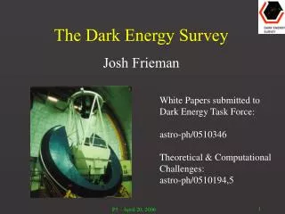
Science of the Dark Energy Survey Josh Frieman Fermilab and the University of Chicago Astronomy 41100 Lecture 2, Oct. 15, 2010
DES Collaboration Meeting Go to: http://astro.fnal.gov/desfall2010/Home.html Science Working group meetings on Tuesday. Plenary sessions Wed-Fri.
Cosmological Constant as Dark Energy Einstein: Zel’dovich and Lemaitre:
Cosmological Constant as Dark Energy Quantum zero-point fluctuations: virtual particles continuously fluctuate into and out of the vacuum (via the Uncertainty principle). Vacuum energy density in Quantum Field Theory: Theory: Data: Pauli Cosmological Constant Problem
Dark Energy: Alternatives to Λ The smoothness of the Universe and the large-scale structure of galaxies can be neatly explained if there was a much earlier epoch of cosmic acceleration that occurred a tiny fraction of a second after the Big Bang: Primordial Inflation Inflation ended, so it was not driven by the cosmological constant. This is a caution against theoretical prejudice for Λ as the cause of current acceleration (i.e., as the identity of dark energy).
Light Scalar Fields as Dark Energy Perhaps the Universe is not yet in its ground state. The `true’ vacuum energy (Λ) could be zero (for reasons yet unknown). Transient vacuum energy can exist if there is a field that takes a cosmologically long time to reach its ground state. This was the reasoning behind inflation. For this reasoning to apply now, we must postulate the existence of an extremely light scalar field, since the dynamical evolution of such a field is governed by JF, Hill, Stebbins, Waga 1995
Scalar Field as Dark Energy(inspired by inflation) • Dark Energy could be due to a very light scalar field j, slowly evolving in a potential, V(j): • Density & pressure: • Slow roll: V(j) j
Scalar Field Dark Energy aka quintessence General features: meff< 3H0 ~ 10-33 eV (w < 0) (Potential > Kinetic Energy) V ~ m22 ~ crit ~ 10-10 eV4 ~ 1028 eV ~ MPlanck V(j) (10–3 eV)4 j 1028 eV Ultra-light particle: Dark Energy hardly clusters, nearly smooth Equation of state: usually, w > 1 and evolves in time Hierarchy problem: Why m/ ~ 1061? Weak coupling: Quartic self-coupling < 10122
The Coincidence Problem Why do we live at the `special’ epoch when the dark energy density is comparable to the matter energy density? matter ~ a-3 DE~ a-3(1+w) a(t) Today
Scalar Field Models & Coincidence `Dynamics’ models (Freezing models) `Mass scale’ models (Thawing models) V V e.g., e– or –n MPl Runaway potentials DE/matter ratio constant (Tracker Solution) Pseudo-Nambu Goldstone Boson Low mass protected by symmetry (Cf. axion)JF, Hill, Stebbins, Waga V() = M4[1+cos(/f)] f ~ MPlanck M ~ 0.001 eV ~ m Ratra & Peebles; Caldwell,etal
PNGB Models • Tilted Mexican hat: M4 • Spontaneous symmetry breaking at scale f • Explicit breaking at scale M • Hierarchy protected by symmetry f Frieman, Hill, Stebbins, Waga 2005
Dynamical Evolution of Freezing vs. Thawing Models Caldwell & Linder Measuring w and its evolution can potentially distinguish between physical models for acceleration 12
Runaway (Tracker) Potentials Typically >> Mplanck today. Must prevent terms of the form V() ~ n+4 / Mplanckn up to large n What symmetry prevents them?
Perturbations of Scalar Field Dark Energy If it evolves in time, it must also vary in space. h = synchronous gauge metric perturbation Fluctuations distinguish this from a smooth “x-matter” or Coble, Dodelson, Frieman 1997 Caldwell et al, 1998
Dark Energy Interactions Couplings to visible particles must be small Carroll 1998 Frieman & Gradwohl 1990, 1992 Couplings cause long-range forces Example: scalar field coupled to massive neutrino Attractive force between lumps of
What about w < 1? The Big Rip • H(t) and a(t) increase with time and diverge in finite time • e.g, for w=-1.1, tsing~100 Gyr • Scalar Field Models: • need to violate null Energy condtion+ p > 0: • for example: • L = ()2 V • Controlling instability requires cutoff at low mass scale • Modified Gravity models • apparently can achieve effective w< –1 without • violating null Energy Condition Caldwell, etal Hoffman, etal
Modified Gravity & Extra Dimensions • 4-dimensional brane in 5-d Minkowski space • Matter lives on the brane • At large distances, gravity can leak offbraneinto • the bulk, infinite 5th dimension Dvali, Gabadadze, Porrati • Acceleration without vacuum energy on the brane, • driven by brane curvature term • Action given by: • Consistency problems: ghosts, strong coupling
Modified Gravity • Weak-field limit: • Consider static source on the brane: • Solution: • In GR, 1/3 would be ½ • Characteristic cross-over scale: • For modes with p<<1/rc: • Gravity leaks off the brane: longer wavelength gravitons free to • propagate into the bulk • Intermediate scales: scalar-tensor theory
Cosmological Solutons • Modified Friedmann equation: • Early times: H>>1/rc: ordinary behavior, decelerated expansion. • Late times: self-accelerating solution for (-) • For we require • At current epoch, deceleration parameter is • corresponds to weff=-0.8
Growth of Perturbations • Linear perturbations approximately satisfy: • Can change growth factor by ~30% relative to GR • Motivates probing growth of structure in addition to expansion rate
Modified Gravity: f(R) This particular realization excluded by solar system tests, but variants evade them: Chameleon models hide deviations from GR on solar system scales
Bolometric Distance Modulus • Logarithmic measures of luminosity and flux: • Define distance modulus: • For a population of standard candles (fixed M), measurements of vs. z, the Hubble diagram, constrain cosmological parameters. flux measure redshift from spectra
Distance Modulus • Recall logarithmic measures of luminosity and flux: • Define distance modulus: • For a population of standard candles (fixed M) with known spectra (K) and known extinction (A), measurements of vs. z, the Hubble diagram, constrain cosmological parameters. denotes passband
K corrections due to redshift SN spectrum Rest-frame B band filter Equivalent restframei band filter at different redshifts (iobs=7000-8500 A)
Absolute vs. Relative Distances • Recall logarithmic measures of luminosity and flux: • If Mi is known, from measurement of mi can infer absolute distance to an object at redshiftz, and thereby determine H0 (for z<<1, dL=cz/H0) • If Mi (and H0) unknown but constant, from measurement of mi can infer distance to object at redshiftz1 relative to object at distance z2: independent of H0 • Use low-redshiftSNe to vertically `anchor’ the Hubble diagram, i.e., to determine
Ia SN Spectra ~1 week after maximum light Filippenko 1997 II Ic Ib
Type Ia Supernovae Thermonuclear explosions of Carbon-Oxygen White Dwarfs White Dwarf accretes mass from or merges with a companion star, growing to a critical mass~1.4Msun (Chandrasekhar) After ~1000 years of slow cooking, a violent explosion is triggered at or near the center, and the star is completely incinerated within seconds In the core of the star, light elements are burned in fusion reactions to form Nickel. The radioactive decay of Nickel and Cobalt makes it shine for a couple of months
General properties: Homogeneous class* of events, only small (correlated) variations Rise time: ~ 15 – 20 days Decay time: many months Bright: MB ~ – 19.5 at peak No hydrogen in the spectra Early spectra: Si, Ca, Mg, ...(absorption) Late spectra: Fe, Ni,…(emission) Very high velocities (~10,000 km/s) SN Ia found in all types of galaxies, including ellipticals Progenitor systems must have long lifetimes Type Ia Supernovae *luminosity, color, spectra at max. light
SN Ia Spectral Homogeneity(to lowest order) from SDSS Supernova Survey
SN2004ar z = 0.06 from SDSS galaxy spectrum Galaxy-subtracted Spectrum SN Ia template
How similar to one another?Some real variations:absorption-line shapes at maximumConnections to luminosity?Matheson, etal, CfA sample
Supernova IaSpectral Evolution Late times Early times Hsiao etal
Layered Chemical Structure provides clues to Explosion physics
SN1998bu Type Ia Multi-band Light curve Extremely few light-curves are this well sampled Suntzeff, etal Jha, etal Hernandez, etal
Luminosity m15 15 days Time Empirical Correlation: Brighter SNeIa decline more slowly and are bluer Phillips 1993
SN Ia Peak Luminosity Empirically correlated with Light-Curve Decline Rate Brighter Slower Use to reduce Peak Luminosity Dispersion Phillips 1993 Peak Luminosity Rate of decline Garnavich, etal
Type Ia SN Peak Brightness as calibrated Standard Candle Peak brightness correlates with decline rate Variety of algorithms for modeling these correlations: corrected dist. modulus After correction, ~ 0.16 mag (~8% distance error) Luminosity Time
Published Light Curves for Nearby Supernovae Low-z SNe: Anchor Hubble diagramTrain Light-curve fittersNeed well-sampled, well-calibrated, multi-band light curves
Carnegie Supernova Project Nearby Optical+ NIR LCs
Correction for Brightness-Decline relation reduces scatter in nearby SN Ia Hubble Diagram Distance modulus for z<<1: Corrected distance modulus is not a direct observable: estimated from a model for light-curve shape Riessetal 1996
Acceleration Discovery Data:High-z SN Team 10 of 16 shown; transformed to SN rest-frame Riessetal Schmidt etal V B+1
Likelihood Analysis This assume Goliath etal 2001
Exercise 5 • Carry out a likelihood analysis of using the High-Z Supernova Data of Riess, etal 1998: use Table 10 above for low-z data and the High-z table above for high-zSNe. Assume a fixed Hubble parameter for the first part of this exercise. • 2nd part: repeat the exercise, but marginalizing over H0 with a flat prior, either numerically or using the analytic method of Goliath etal. • Errors: assume intrinsic dispersion of and fit dispersions from the tables and dispersion due to peculiar velocity from Kessler etal (0908.4274), Eqn. 28, with