Motivation

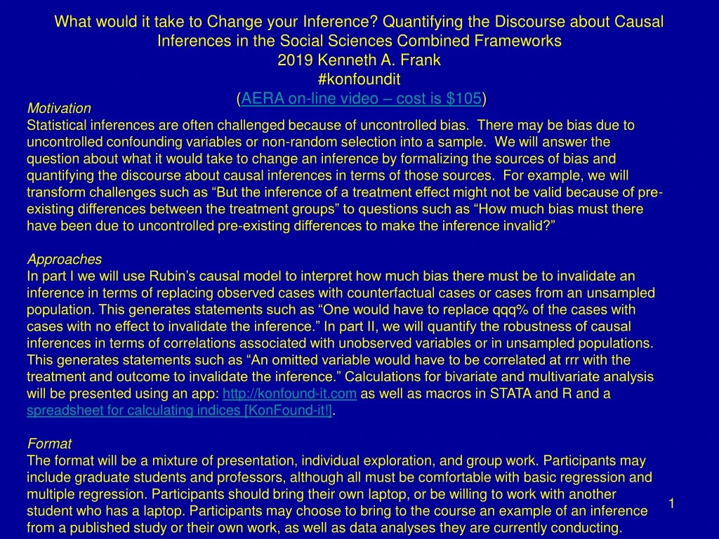
1. What would it take to Change your Inference? Quantifying the Discourse about Causal Inferences in the Social Sciences Combined Frameworks 2019 Kenneth A. Frank #konfoundit (AERA on-line video – cost is $105) Motivation Statistical inferences are often challenged because of uncontrolled bias. There may be bias due to uncontrolled confounding variables or non-random selection into a sample. We will answer the question about what it would take to change an inference by formalizing the sources of bias and quantifying the discourse about causal inferences in terms of those sources. For example, we will transform challenges such as “But the inference of a treatment effect might not be valid because of pre-existing differences between the treatment groups” to questions such as “How much bias must there have been due to uncontrolled pre-existing differences to make the inference invalid?” Approaches In part I we will use Rubin’s causal model to interpret how much bias there must be to invalidate an inference in terms of replacing observed cases with counterfactual cases or cases from an unsampled population. This generates statements such as “One would have to replace qqq% of the cases with cases with no effect to invalidate the inference.” In part II, we will quantify the robustness of causal inferences in terms of correlations associated with unobserved variables or in unsampled populations. This generates statements such as “An omitted variable would have to be correlated at rrr with the treatment and outcome to invalidate the inference.” Calculations for bivariate and multivariate analysis will be presented using an app: http://konfound-it.com as well as macros in STATA and R and a spreadsheet for calculating indices [KonFound-it!]. Format The format will be a mixture of presentation, individual exploration, and group work. Participants may include graduate students and professors, although all must be comfortable with basic regression and multiple regression. Participants should bring their own laptop, or be willing to work with another student who has a laptop. Participants may choose to bring to the course an example of an inference from a published study or their own work, as well as data analyses they are currently conducting.

2. https://msu.edu/~kenfrank/research.htm

3. Motivation Inferences uncertain it’s causal inference not determinism Do you have enough information to make a decision? Instead of “you didn’t control for xxx” Personal: Granovetter to Fernandez What would xxx have to be to change your inference Promotes scientific discourse Informs pragmatic policy

4. overview Replacement Cases Framework (40 minutes to reflection) Thresholds for inference and % bias to invalidate and inference The counterfactual paradigm Application to concerns about non-random assignment to treatments Application to concerns about non-random sample Reflection (10 minutes) Examples of replacement framework Internal validity example: Effect of kindergarten retention on achievement (40 minutes to break) External validity example: effect of Open Court curriculum on achievement Review and Reflection Extensions Extensions of the framework Exercise and break (20 minutes) Correlational Framework (25 minutes to exercise) How regression works Impact of a Confounding variable Internal validity: Impact necessary to invalidate an inference Example: Effect of kindergarten retention on achievement Exercise (25 minutes) External validity (30 minutes) combining estimates from different populations example: effect of Open Court curriculum on achievement Conclusion (10 minutes)

5. Quick Survey Can you make a causal inference from an observational study?

6. Answer: Quantifying the Discourse Can you make a causal inference from an observational study? Of course you can. You just might be wrong. It’s causal inference, not determinism. But what would it take for the inference to be wrong?

7. I: Replacement of Cases Framework How much bias must there be to invalidate an inference? Concerns about Internal Validity • What percentage of cases would you have to replace with counterfactual cases (with zero effect) to invalidate the inference? Concerns about External Validity • What percentage of cases would you have to replace with cases from an unsampled population (with zero effect) to invalidate the inference?

8. What Would It Take to Change an Inference? Using Rubin’s Causal Model to Interpret the Robustness of Causal Inferences Abstract We contribute to debate about causal inferences in educational research in two ways. First, we quantify how much bias there must be in an estimate to invalidate an inference. Second, we utilize Rubin’s causal model (RCM) to interpret the bias necessary to invalidate an inference in terms of sample replacement. We apply our analysis to an inference of a positive effect of Open Court Curriculum on reading achievement from a randomized experiment, and an inference of a negative effect of kindergarten retention on reading achievement from an observational study. We consider details of our framework, and then discuss how our approach informs judgment of inference relative to study design. We conclude with implications for scientific discourse. Keywords: causal inference; Rubin’s causal model; sensitivity analysis; observational studies Frank, K.A., Maroulis, S., Duong, M., and Kelcey, B. 2013.  What would it take to Change an Inference?: Using Rubin’s Causal Model to Interpret the Robustness of Causal Inferences.   Education, Evaluation and Policy Analysis.  Vol 35: 437-460.http://epa.sagepub.com/content/early/recent

9. % bias necessary to invalidate the inference { }

10. Quantifying the Discourse: Formalizing Bias Necessary to Invalidate an Inference δ =a population effect, =the estimated effect, and δ# =the threshold for making an inference An inference is invalid if: (1) An inference is invalid if the estimate is greater than the threshold while the population value is less than the threshold. Defining bias as -δ, (1) implies an inference is invalid if and only if: Expressed as a proportion of the estimate, inference invalid if:

11. The full Algebra for Exceeding a Threshold

12. δ# % bias necessary to invalidate the inference { } δ#

13. Interpretation of % Bias to Invalidate an Inference % Bias is intuitive Relates to how we think about statistical significance Better than “highly significant” or “barely significant” But need a framework for interpreting

14. Sensitivity vs Robustness Sensitivity of estimate assess how estimates change as a result of alternative analyses Different covariates Different sub-samples Different estimation techniques Robustness of the inference quantifies what it would take to change an inference based on hypothetical data or conditions Unobserved covariates Unobserved samples

15. Framework for Interpreting % Bias to Invalidate an Inference: Rubin’s Causal Model and the Counterfactual • I have a headache • I take an aspirin (treatment) • My headache goes away (outcome) • Q) Is it because I took the aspirin? • We’ll never know – it is counterfactual – for the individual • This is the Fundamental Problem of Causal Inference

16. Approximating the Counterfactual with Observed Data But how well does the observed data approximate the counterfactual? Difference between counterfactual values and observed values for the control implies the treatment effect of 1 8 9 10 1 1 1 3 4 5 6 4.00 9 is overestimated as 6 using observed control cases with mean of 4

17. Using the Counterfactual to Interpret % Bias to Invalidate the Inference: Replacement with Average Values How many cases would you have to replace with zero effect counterfactuals to change the inference? Assume threshold is 4 (δ# =4): 1- δ# / =1-4/6=.33 =(1/3) 6 6 6 0 0 0 7 7 7 3 4 5 7 7 7 4 6 9 5 The inference would be invalid if you replaced 33% (or 1 case) with counterfactuals for which there was no treatment effect. New estimate=(1-% replaced) +%replaced(no effect)= (1-%replaced) =(1-.33)6=.66(6)=4

18. Which Cases to Replace? Think of it as an expectation: if you randomly replaced 1 case, and repeated 1,000 times, on average the new estimate would be 4 Assumes constant treatment effect conditioning on covariates and interactions already in the model Assumes cases carry equal weight

19. % bias necessary to invalidate the inference { } δ# To invalidate the inference, replace 33% of cases with counterfactual data with zero effect

20. Review & Reflection Review of Framework Pragmatism  thresholds How much does an estimate exceed the threshold  % bias to invalidate the inference Interpretation: Rubin’s causal model • internal validity: % bias to invalidate  number of cases that must be replaced with counterfactual cases (for which there is no effect) Reflect Which part is most confusing to you? Is there more than one interpretation? Discuss with a partner or two

21. Example of Internal Validity from Observational Study : The Effect of Kindergarten Retention on Reading and Math Achievement(Hong and Raudenbush 2005) • 1. What is the average effect of kindergarten retention policy? (Example used here) • Should we expect to see a change in children’s average learning outcomes if a school changes its retention policy? • Propensity based questions (not explored here) • 2. What is the average impact of a school’s retention policy on children who would be promoted if the policy were adopted? • Use principal stratification. • Hong, G. and Raudenbush, S. (2005). Effects of Kindergarten Retention Policy on Children’s Cognitive Growth in Reading and Mathematics. Educational Evaluation and Policy Analysis. Vol. 27, No. 3, pp. 205–224

22. Data • Early Childhood Longitudinal Study Kindergarten cohort (ECLSK) • US National Center for Education Statistics (NCES). • Nationally representative • Kindergarten and 1st grade • observed Fall 1998, Spring 1998, Spring 1999 • Student • background and educational experiences • Math and reading achievement (dependent variable) • experience in class • Parenting information and style • Teacher assessment of student • School conditions • Analytic sample (1,080 schools that do retain some children) • 471 kindergarten retainees • 7,168 promoted students

23. Estimated Effect of Retention on Reading Scores(Hong and Raudenbush)

24. Possible Confounding Variables(note they controlled for these) • Gender • Two Parent Household • Poverty • Mother’s level of Education (especially relevant for reading achievement) • Extensive pretests • measured in the Spring of 1999 (at the beginning of the second year of school) • standardized measures of reading ability, math ability, and general knowledge; • indirect assessments of literature, math and general knowledge that include aspects of a child’s process as well as product; • teacher’s rating of the child’s skills in language, math, and science

25. Obtain df, Estimated Effect and Standard Error Standard error=.68 Estimated effect ( ) = -9.01 n=7168+471=7639; df > 500, t critical=-1.96 From: Hong, G. and Raudenbush, S. (2005). Effects of Kindergarten Retention Policy on Children’s Cognitive Growth in Reading and Mathematics. Educational Evaluation and Policy Analysis. Vol. 27, No. 3, pp. 205–224

26. # of covariates Page 215 Df used in model=207+14+2=223 Add 2 to include the intercept and retention

27. Calculating % Bias to Invalidate the Inference 1) Calculate threshold δ# Estimated effect is statistically significant if: |Estimated effect| /standard error > |tcritical| |Estimated effect| > |tcritical |x standard error=δ # |Estimated effect| > 1.96 x .68 = 1.33=δ # 2) Record =|Estimated effect|= 9.01 3) % bias to invalidate the inference is 1- δ #/ =1-.1.33/9.01=.85 85% of the estimate would have to be due to bias to invalidate the inference You would have to replace 85% of the cases with counterfactual cases with 0 effect of retention on achievement to invalidate the inference

28. In R Shiny app KonFound-it!(konfound-it.com/) Estimated effect Standard error Number of observations Number of covariates Take out your phone and try it!!!

29. % Bias necessary to invalidate inference = =1-1.33/9.01=85% 85% of the estimate must be due to bias to invalidate the inference. 85% of the cases must be replaced with null hypothesis cases to invalidate the inference Estimated Effect δ# Threshold

30. Using the Counterfactual to Interpret % Bias to Invalidate the Inference: Replacement with Average Values How many cases would you have to replace with zero effect counterfactuals to change the inference? Assume threshold is 4 (δ# =4): 1- δ# / =1-4/6=.33 =(1/3) 6 6 6 0 0 0 7 7 7 3 4 5 7 7 7 4 6 9 5 The inference would be invalid if you replaced 33% (or 1 case) with counterfactuals for which there was no treatment effect. New estimate=(1-% replaced) +%replaced(no effect)= (1-%replaced) =(1-.33)6=.66(6)=4

31. Example Replacement of Cases with Counterfactual Data to Invalidate Inference of an Effect of Kindergarten Retention Counterfactual: No effect Retained Promoted Original cases that were not replaced Replacement counterfactual cases with zero effect Original distribution

32. Interpretation 1) Consider test scores of a set of children who were retained that are considerably lower (9 points) than others who were candidates for retention but who were in fact promoted. No doubt some of the difference is due to advantages the comparable others had before being promoted. But now to believe that retention did not have an effect one must believe that 85% of those comparable others would have enjoyed most (7.2) of their advantages whether or not they had been retained. This is even after controlling for differences on pretests, mother’s education, etc. 2a) The inference is invalid if we replace 85% cases with cases in which an omitted variable is perfectly correlated with kindergarten retention. 2b) The inference is invalid if we replace 85% of the cases with cases in which an omitted variable is perfectly correlated with the achievement. 3) Could 85% of the children have manifest an effect because of unadjusted differences (even after controlling for prior achievement, motivation and background) rather than retention itself?

33. Which Cases to Replace? Graphics are rigged to make p =.06 Generally: thought experiment of repeating replacement 1,000 times. Average of new estimates will be at the threshold for inference If data are weighted (sample weights, IPTW, HLM, Logistic), then if you remove a unit with case weight of 3, then you replace with a unit with a case weight of 3

34. Evaluation of % Bias Necessary to Invalidate Inference 50% cut off– for every case you remove, I get to keep one Compare bias necessary to invalidate inference with bias accounted for by background characteristics 1% of estimated effect accounted for by background characteristics (including mother’s education), once controlling for pretests e.g. estimate of retention before controlling for mother’s education is -9.1, after controlling for mother’s education it is -9.01, a change of .1 (or about 1% of the final estimate. The estimate would have to change another 85% to invalidate the inference. More than 85 times more unmeasured bias necessary to invalidate the inference Compare with % bias necessary to invalidate inference in other studies: Use correlation metric Adjusts for differences in scale

35. % Bias Necessary to Invalidate Inference based on Correlationto Compare across Studies t taken from HLM: =-9.01/.68=-13.25 n is the sample size q is the number of parameters estimated Where t is critical value for df>200 % bias to invalidate inference=1-(-.023)/(-.152)=85% Accounts for changes in regression coefficient and standard error Because t(r)=t(β)

36. r % bias necessary to invalidate the inference { r } r#

37. r Accounts for Changes in R2 and Changes in Standard error: T(r) = T(β/se(β)). So if we work in the correlation metric it inherently accounts for changes in R2. Good to use for comparison across studies or comarison with bias accounted for by observed covariates within study For comparison, see Oster, E. (2019). Unobservable selection and coefficient stability: Theory and evidence. Journal of Business & Economic Statistics, 37(2), 187-204.

38. Compare with Bias other Observational Studies

39. % Bias to Invalidate versus p-value: a better language? Kindergarten Retention *** Catholic Schools ** * Df=973 based on Morgan’s analysis of Catholic school effects, Functional form not sensitive to df

40. Beyond *, **, and *** • P values • sampling distribution framework • Must interpret relative to standard errors • Information lost for modest and high levels of robustness • % bias to invalidate • counterfactual framework • Interpret in terms of case replacement • Information along a continuous scale

42. % Bias to Invalidate Inference for Observational StudiesOn-line EEPA July 24-Nov 15 2012 Kindergarten retention effect

43. Konfound-it.com R and STATA

44. In R: Pkonfound(published example) install.packages("konfound") library(konfound) pkonfound(est_eff = -9.01, std_err = .68, n_obs = 7639, n_covariates = 223) USE THIS IGNORE FOR NOW

45. Sensitivity on Regression Run in R: Konfound (data in R) data <- read.table(url("https://msu.edu/~kenfrank/p025b.txt"), header = T) model <- lm(Y1 ~ X1 + X4, data = data) model konfound(model, X1) USE THIS IGNORE FOR NOW

46. In STATA • . ssc install konfound • . ssc install moss • . ssc install matsort • . ssc install indeplist • . pkonfound -9.01 .68 7639 223 • . /* pkonfound estimate standard_error n number_of_covariates */ IGNORE FOR NOW USE THIS

47. Step 1: search konfound in the Viewer window Step 2: click on the link, you get this window Step 3: click “click here to install” to install it!

48. Sensitivity on Regression Run in STATA . use https://msu.edu/~kenfrank/p025b.dta, clear     . regress y1 x1 x4     . konfound x1

49. Exercise 1 : % Bias necessary to Invalidate an Inference for Internal Validity • Take an example from an observational study (your own data, the toy example, or a published example) Calculate the % bias necessary to invalidate the inference (using konfound or pkonfound) • [ignore output for correlation based approach with impact] • Interpret the % bias in terms of sample replacement • What are the possible sources of bias? • Would they all work in the same direction? • What happens if you change the • sample size • # of covariates • standard error • Debate your inference with a partner

50. Approximating the Unsampled Population with Observed Data from an RCT (External Validity) How many cases would you have to replace with cases with zero effect to change the inference? Assume threshold is: δ# =4: 1- δ# / =1-4/6=.33 =(1/3) 9 10 11 3 4 5 7 7 7 7 7 7 ´ 0 6 4 Texas Notre Dame