Download
1 / 24
240 likes | 315 Views
Rainfall Measurement. Rainfall measurement. Rain gauge (1 hr) High wind, low rain rate (evaporation) Spatially localized, temporally moderate Radar reflectivity (6 min) Attenuation, not ground measure Spatially integrated, temporally fine Cloud top temp. (satellite, ca 12 hrs)

E N D
Rainfall measurement Rain gauge (1 hr) High wind, low rain rate (evaporation) Spatially localized, temporally moderate Radar reflectivity (6 min) Attenuation, not ground measure Spatially integrated, temporally fine Cloud top temp. (satellite, ca 12 hrs) Not directly related to precipitation Spatially integrated, temporally sparse Distrometer (drop sizes, 1 min) Expensive measurement Spatially localized, temporally fine
Basic relations Rainfall rate: v(D) terminal velocity for drop size D N(t) number of drops at time t f(D) pdf for drop size distribution Gauge data: g(w) gauge type correction factor w(t) meteorological variables such as wind speed
Basic relations, cont. Radar reflectivity: Observed radar reflectivity:
Structure of model Data: [G|N(D),qG] [Z|N(D),qZ] Processes: [N|mN,qN] [D|xt,qD] log GARCH LN Temporal dynamics: [mN(t)|qm] AR(1) Model parameters: [qG,qZ,qN,qm,qD|qH] Hyperparameters: qH
The Kalman filter Gauss (1795) least squares Kolmogorov (1941)-Wiener (1942) dynamic prediction Follin (1955) Swerling (1958) Kalman (1960) recursive formulation prediction depends on how far current state is from average Extensions
A state-space model Write the forecast anomalies as a weighted average of EOFs (computed from the empirical covariance) plus small-scale noise. The average develops as a vector autoregressive model:
Model assessment Difference from current forecast of Previous forecast Kalman filter Satellite data assimilated
Statistical analysis of computer code output Often the process model is expensive to run (in time, at least), especially if different runs needed for MCMC Need to develop real-time approximation to process model Kalman filter is a dynamic linear model approximation SACCO is an alternative Bayesian approach
Basic framework An emulator is a random (Gaussian) process (x) approximating the process model for input x in Rm. Prior mean m(x) = h(x)T Prior covariance Run the model at n input values to get n output values, so
The emulator Integrating out and 2 we get where q = dim() and where t(x)T = (c(x,x1),…,c(x,xn)) m** is the emulator, and we can also calculate its variance
An example y=7+x+cos(2x) q=1, hT(x)=(1 x) n=5
Conclusions Model assessment constraints: • amount of data • data quality • ease of producing model runs • degree of misalignment Ideally the model should have • similar first and second order properties to the data • similar peaks and troughs to data (or simulations based on the data)