Download

1 / 58
670 likes | 749 Views
Explore the world of image restoration, from understanding degradation models to applying spatial filters for noise reduction. Learn about noise types, estimation techniques, and adaptive filters for enhanced image quality.

E N D
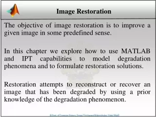
Preview • Goal of image restoration • Improve an image in some predefined sense • Difference with image enhancement ? • Features • Image restoration v.s image enhancement • Objective process v.s. subjective process • A prior knowledge v.s heuristic process • A prior knowledge of the degradation phenomenon is considered • Modeling the degradation and apply the inverse process to recover the original image
Preview (cont.) • Target • Degraded digital image • Sensor, digitizer, display degradations are less considered • Spatial domain approach • Frequency domain approach
Outline • A model of the image degradation / restoration process • Noise models • Restoration in the presence of noise only– spatial filtering • Periodic noise reduction by frequency domain filtering • Linear, position-invariant degradations • Estimating the degradation function • Inverse filtering
A model of the image degradation/restoration process g(x,y)=f(x,y)*h(x,y)+h(x,y) G(u,v)=F(u,v)H(u,v)+N(u,v)
Noise models 雜訊模型 • Source of noise • Image acquisition (digitization) • Image transmission • Spatial properties of noise • Statistical behavior of the gray-level values of pixels • Noise parameters, correlation with the image • Frequency properties of noise • Fourier spectrum • Ex. white noise (a constant Fourier spectrum)
Noise probability density functions • Noises are taken as random variables • Random variables • Probability density function (PDF)
Gaussian noise • Math. tractability in spatial and frequency domain • Electronic circuit noise and sensor noise mean variance Note:
Gaussian noise (PDF) 70% in [(m-s), (m+s)] 95% in [(m-2s), (m+2s)]
Uniform noise • Less practical, used for random number generator Mean: Variance:
Impulse (salt-and-pepper) nosie • Quick transients, such as faulty switching during imaging If either Pa or Pb is zero, it is called unipolar. Otherwise, it is called bipoloar. • In practical, impulses are usually stronger than image • signals. Ex., a=0(black) and b=255(white) in 8-bit image.
Test for noise behavior • Test pattern Its histogram: 0 255
Periodic noise • Arise from electrical or electromechanical interference during image acquisition • Spatial dependence • Observed in the frequency domain
Sinusoidal noise: Complex conjugate pair in frequency domain
Estimation of noise parameters • Periodic noise • Observe the frequency spectrum • Random noise with unknown PDFs • Case 1: imaging system is available • Capture images of “flat” environment • Case 2: noisy images available • Take a strip from constant area • Draw the histogram and observe it • Measure the mean and variance
Observe the histogram uniform Gaussian
Measure the mean and variance • Histogram is an estimate of PDF Gaussian: m, s Uniform: a, b
Outline • A model of the image degradation / restoration process • Noise models • Restoration in the presence of noise only – spatial filtering • Periodic noise reduction by frequency domain filtering • Linear, position-invariant degradations • Estimating the degradation function • Inverse filtering
Additive noise only g(x,y)=f(x,y)+h(x,y) G(u,v)=F(u,v)+N(u,v)
Spatial filters for de-noising additive noise • Skills similar to image enhancement • Mean filters • Order-statistics filters • Adaptive filters
Mean filters • Arithmetic mean • Geometric mean Window centered at (x,y)
Noisy Gaussian original m=0 s=20 Arith. mean Geometric mean
Mean filters (cont.) • Harmonic mean filter • Contra-harmonic mean filter Q=-1, harmonic Q=0, airth. mean Q=+, ?
Pepper Noise 黑點 Salt Noise 白點 Contra- harmonic Q=-1.5 Contra- harmonic Q=1.5
Wrong sign in contra-harmonic filtering Q=1.5 Q=-1.5
Order-statistics filters • Based on the ordering(ranking) of pixels • Suitable for unipolar or bipolar noise (salt and pepper noise) • Median filters • Max/min filters • Midpoint filters • Alpha-trimmed mean filters
Order-statistics filters • Median filter • Max/min filters
bipolar Noise Pa = 0.1 Pb = 0.1 3x3 Median Filter Pass 1 3x3 Median Filter Pass 2 3x3 Median Filter Pass 3
Salt noise Pepper noise Min filter Max filter
Order-statistics filters (cont.) • Midpoint filter • Alpha-trimmed mean filter • Delete the d/2 lowest and d/2 highest gray-level pixels Middle (mn-d) pixels
Uniform noise Left + Bipolar Noise Pa = 0.1 Pb = 0.1 m=0 s2=800 5x5 Arith. Mean filter 5x5 Geometric mean 5x5 Median filter 5x5 Alpha-trim. Filter d=5
Adaptive filters • Adapted to the behavior based on the statistical characteristics of the image inside the filter region Sxy • Improved performance v.s increased complexity • Example: Adaptive local noise reduction filter
Adaptive local noise reduction filter • Simplest statistical measurement • Mean and variance • Known parameters on local region Sxy • g(x,y): noisy image pixel value • s2h: noise variance (assume known a prior) • mL : local mean • s2L: local variance
Adaptive local noise reduction filter (cont.) • Analysis: we want to do • If s2h is zero, return g(x,y) • If s2L> s2h , return value close to g(x,y) • If s2L= s2h , return the arithmetic mean mL • Formula
Gaussian noise Arith. mean 7x7 m=0 s2=1000 Geometric mean 7x7 adaptive
Outline • A model of the image degradation / restoration process • Noise models • Restoration in the presence of noise only – spatial filtering • Periodic noise reduction by frequency domain filtering • Linear, position-invariant degradations • Estimating the degradation function • Inverse filtering
Periodic noise reduction • Pure sine wave • Appear as a pair of impulse (conjugate) in the frequency domain
Periodic noise reduction (cont.) • Bandreject filters • Bandpass filters • Notch filters • Optimum notch filtering
Bandreject filters * Reject an isotropic frequency ideal Butterworth Gaussian
noisy spectrum filtered bandreject
Bandpass filters • Hbp(u,v)=1- Hbr(u,v)
Notch filters • Reject(or pass) frequencies in predefined neighborhoods about a center frequency ideal Butterworth Gaussian
Horizontal Scan lines Notch pass DFT Notch pass Notch reject
Outline • A model of the image degradation / restoration process • Noise models • Restoration in the presence of noise only – spatial filtering • Periodic noise reduction by frequency domain filtering • Linear, position-invariant degradations • Estimating the degradation function • Inverse filtering
A model of the image degradation /restoration process g(x,y)=f(x,y)*h(x,y)+h(x,y) G(u,v)=F(u,v)H(u,v)+N(u,v) If linear, position-invariant system
Linear, position-invariant degradation Properties of the degradation function H • Linear system • H[af1(x,y)+bf2(x,y)]=aH[f1(x,y)]+bH[f2(x,y)] • Position(space)-invariant system • H[f(x,y)]=g(x,y) • H[f(x-a, y-b)]=g(x-a, y-b) • c.f. 1-D signal • LTI (linear time-invariant system)
Linear, position-invariant degradation model • Linear system theory is ready • Non-linear, position-dependent system • May be general and more accurate • Difficult to solve compuatationally • Image restoration: find H(u,v) and apply inverse process • Image deconvolution