Download
1 / 40
400 likes | 1.04k Views
CHRONUX functions for signal conditioning: removing line elements (eg. 60 Hz). rmlinescremoves significant sine waves from data (continuous data).usage: data=rmlinesc(data,params,p,plt,f0)data (data as a matrix times x channels or a single vector) params structure containing parameters - ha

E N D
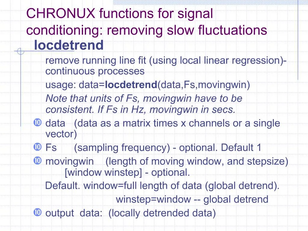
1. CHRONUX functions for signal conditioning: removing slow fluctuations locdetrend
remove running line fit (using local linear regression)-continuous processes
usage: data=locdetrend(data,Fs,movingwin)
Note that units of Fs, movingwin have to be consistent. If Fs in Hz, movingwin in secs.
data (data as a matrix times x channels or a single vector)
Fs (sampling frequency) - optional. Default 1
movingwin (length of moving window, and stepsize) [window winstep] - optional.
Default. window=full length of data (global detrend).
winstep=window -- global detrend
output data: (locally detrended data)
2. CHRONUX functions for signal conditioning: removing line elements (eg. 60 Hz) rmlinesc
removes significant sine waves from data (continuous data).
usage: data=rmlinesc(data,params,p,plt,f0)
data (data as a matrix times x channels or a single vector)
params structure containing parameters - has the
following fields: tapers, Fs, fpass, pad.
Note that units of Fs, fpass have to be consistent (eg. Hz)
tapers: parameters for calculating Slepian tapers,
N?tW and K, the number of tapers.
fpass: frequency band to be used
pad: padding factor for the FFT
p: p-value for F-test
f0: frequencies of lines to be removed if unspecified the F statistic is used to determine the appropriate lines for removal
output data: (data with significant lines removed)
5. Human Electrocorticography (EcoG) Recordings obtained from a patient with intractable epilepsy undergoing evaluation for surgery (all procedures involving patients were approved by the IRB of the Weill Medical College of Cornell University, NYC).
60 electrodes are located on the surface of the cortex, under the dura: 6 electrodes/strip, 5 strips/hemisphere. In addition, 16 depth electrodes (wires) are located in the middle-temporal lobe (8 wires/hemisphere).
Recordings made while the patient performed a simple maze navigation task.
Sampling Rate: 500 Hz
Sample Duration: 8 seconds
6. 60 Hz line noise (50 Hz in Europe).
Capacitative and inductive coupling to the alternating current used in the power distribution supplying the hospital room, OR, laboratory. Sources: room lighting, TVs, other medical equipment.
Slow drifts in baseline voltage. Electrostatic charge distributions change as patient moves in the hospital bed.
Transient voltage spikes generated by capacitative discharge of electrostatic charges built up around patient.
Heart EKG, chest movements. Human Electrocorticography (EcoG): Problems when recording at bedside.
10. Alternative Approach for Signal Conditioning Combine SVD with spectral analysis
Look for the subspace that does not contain noise and major artifacts
Reconstruct a set of signals from the subspace for further analysis
11. >> EcoG
Loads EcoG_dataV6.mat should be compatible with all versions of MATLAB, 6 and above
Defines variables: ATR, ATL, PTR, PRL, DFL, DFR, etc.
Generates two figures: 1) voltage traces for all channels from left hemisphere; 2) same for right hemisphere.
8 seconds of data shown
14. >> return Generates figure showing one channel of recording for each cortical region in right hemisphere
16. >> return
(or uparrow) locdetrend is run on each channel
Fs=500 Hz (sampling rate)
movingwin = [1. 0.5]
window length = 1 second
window step = 0.5 seconds
Ex. dfrontal(:,13) = locdetrend(frontal(:,13),Fs,movingwin);
generates figure showing a detrended channel, dfrontal(:,13) and the original time series, frontal(:,13)
18. >> Locdetrend_Demo
locdetrend is run on a channel selected from the frontal lobe EcoG leads.
movingwin: you will be prompted for
window length
window step
Generates a sequence of figures illustrating windowed samples of EcoG signal, the signal mean and the best fitting line to the sample.
Also shows how the results of the linear regression are locally weighted and combined into a estimate of the entire 8 second signal.
19. How much detrending should be done? That is, how does one choose the window and winstep parameter values? The intermediate stage of detrending acts like a low-pass filter.
The longer the window, the �smoother� the signal will be that you subtract from your original, and hence, the more high-frequency content will be preserved in the residual.
While its important to smooth the signal before subtracting from the original, remember not to smother it.
Simple moving averages (low-pass filtering operations) produce significant distortions.
20. >> Remove_Lines Multi-taper power spectra calculated for one, right hemisphere dorsal-frontal channel, DFR, after detrending.
[S,f] = mtspectrumc(dDFR,params)
with
Ktapers=8; NW=(Ktapers+1)/2
params.tapers=[NW Ktapers]
params.pad=5
params.Fs=500
params.fpass=[0 params.Fs/2]
22. Line-removal from one channel, dDFR. >> return rmlinesc(dDFR,params,.05,�y�)
with parameters
params.tapers = [ 4.5 8]
params.Fs = 500
params.fpass = [ 0 params.Fs/2]
params.pad = 5
Note that we will use the result of the F-test to determine which frequencies to remove (f0 is not explicitly specified), thus we must modify the p-value to compensate for multiple comparisons across many frequencies. This is done automatically in rmlinesc.
24. Line-removal from one channel, dDFR. >> return rmlinesc(dDFR,params,.5,�y�)
with
params.tapers = [ 4.5 8]
params.Fs = 500
params.fpass = [ 0 params.Fs/2]
params.pad = 5
Here, an unusually low value is chosen for the F-statistic (by choosing p to be very large, 0.5).
26. Line-removal from one channel, dDFR. >> return rmlinesc(dDFR,params,.05,�y�,f0)
with
f0 = 60 Hz
params.tapers = [ 2.5 4]
params.Fs = 500
params.fpass = [ 0 params.Fs/2]
params.pad = 5
Here a single frequency is examined, so p-value = 0.05. No correction is made for multiple comparisons.
28. Line-removal from one channel, dDFR. >> return cleanDFR1= rmlinesc(dDFR,params,.05,�y�,f0)
with
f0 = 60.025
Then, cleanDFR2= rmlinesc(cleanDFR1,params,.05,�y�,f0)
with
f0 = 180.075
Then, cleanDFR3= rmlinesc(cleanDFR2,params,.05,�y�,f0)
with
f0 = 199.88
31. Line-removal from one channel, dDFR. >> return cleanDFR= rmlinesc(dDFR,params,.05,�y�,f0)
with
f0 = 60.025
But now with params.pad = 1, instead of params.pad = 5.
32. Alternative Approach for Signal Conditioning Combine SVD with spectral analysis
Look for the subspace that does not contain noise and major artifacts
Reconstruct a set of signals from the subspace for further analysis
>>DeNoise_SVD
34. Multivariate analysis FrontalR is a rectangular matrix, 4000 rows (times samples) x 12 columns (recording channels)
in MATLAB, we can produce a factorization of this matrix by singular value decomposition with:
[U,S,V] = svd(FrontalR,0);
Columns in U are the temporal modes of FrontalR
Columns in V are the �spatial� modes of FrontalR
diag(S) gives the singular values of FrontalR
�economy size� decomposition
>> return
36. >> return Multi-taper power spectra calculated for each of the temporal modes in U
[US(:,1),f] = mtspectrumc(U(:,1),params)
with
Ktapers=20; NW=(Ktapers+1)/2
params.tapers=[NW Ktapers]
params.pad=5
params.Fs=500
params.fpass=[0 params.Fs/2]
38. We drop the first two temporal modes and construct a set of signals from the remaining modes.
U(3:end,3:end)*S(3:end,3:end)*V(3:end,3:end)'
= FrontalRsvd
>> Hit UPARROW or type return
40. Note that neither locdetrend nor rmlinesc were used in this approach to signal conditioning.
Yet the slow, large fluctuations in voltage were removed as well as all the line elements at 60.025, 180.075 and 199.88 Hz.
Approach is more useful as a demonstration of SVD than as a method for removing the electrical artifacts common in EcoG recordings.
41. >> DeNoise_Demo
evaluate how noise and denoising alters the time-frequency structure of EcoG and EEG signals. You will be prompted to choose a region of the cortex to examine.
1 � frontal (24 channels)
2 � parietal (12 channels)
3 � temporal (24 channels)
4 � medial-temporal (16 channels)
You will be prompted to either detrend or not detrend (Y/N).
If �Y�, locdetrend will be run; you will be prompted for:
Window length
Window step
You will be prompted to either remove line noise or not (Y/N).
If �Y�, rmlinesc will be run; you will be prompted for:
Number of tapers to be used for spectral analysis; careful, a large number of tapers could tax limited computer memory
Padding factor; good value to choose � >2.
p-value for significance testing of harmonics; Bonferroni correction is done automatically.
Singular value decomposition is done on the brain region�s channel set. The data are either denoised or not, based on your choices.
A plot is generated of the spectra of the first 5 temporal modes.