Download
1 / 45
561 likes | 1.31k Views
1. 1. 2. 0. -1. 1. 0. 2. 0. 0. -2. 0. 1. -1. -2. 0. -1. -1. Sobel Edge Detection: Gradient Approximation. Note anisotropy of edge finding. Horizontal diff. Vertical diff. Sobel.

E N D
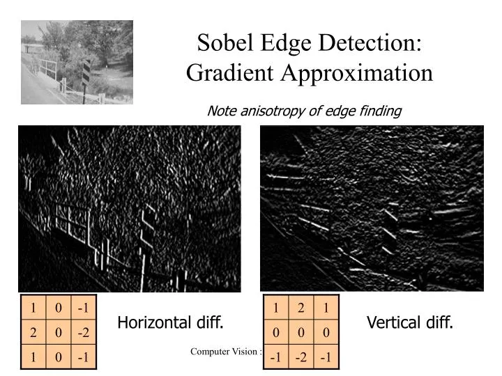
1 1 2 0 -1 1 0 2 0 0 -2 0 1 -1 -2 0 -1 -1 Sobel Edge Detection: Gradient Approximation Note anisotropy of edge finding Horizontal diff. Vertical diff. Computer Vision : CISC 4/689
Sobel • These can then be combined together to find the absolute magnitude of the gradient at each point and the orientation of that gradient. The gradient magnitude is given by: • an approximate magnitude is computed using: which is much faster to compute. • The angle of orientation of the edge (relative to the pixel grid) giving rise to the spatial gradient is given by: In this case, orientation 0 is taken to mean that the direction of maximum contrast from black to white runs from left to right on the image, and other angles are measured anti-clockwise from this. Computer Vision : CISC 4/689
Derivative of Gaussian Computer Vision : CISC 4/689
Smoothing and Differentiation • Issue: noise • smooth before differentiation • two convolutions: to smooth, then differentiate? • actually, no - we can use a derivative of Gaussian filter • because differentiation is convolution, and convolution is associative Computer Vision : CISC 4/689
Another way to detect an extremal first derivative is to look for a zero second derivative the Laplacian Bad idea to apply a Laplacian without smoothing smooth with Gaussian, apply Laplacian this is the same as filtering with a Laplacian of Gaussian filter Now mark the zero points where there is a sufficiently large (first) derivative, and enough contrast The Laplacian of Gaussian Computer Vision : CISC 4/689
Marr-Hildreth operator • The Laplacian is linear and rotationally symmetric. Thus, we search for the zero crossings of the image that is first smoothed with a Gaussian mask and then the second derivative is calculated; or we can convolve the image with the Laplacian of the Gaussian, also known as the LoG operator; • This defines the Marr-Hildreth operator. • One can also get a shape similar to G'' by taking the difference of two Gaussians having different standard deviations. A ratio of standard deviations of 1:1.6 will give a close approximation to .This is known as the DoG operator (Difference of Gaussians), or the Mexican Hat Operator. • Still sensitive to noise. Computer Vision : CISC 4/689
Step edge detection: 2nd-Derivative Operators • Method: 2nd derivative is 0 for 1st-derivative extrema, so find “zero-crossings” • Laplacian Isotropic (finds edges regardless of orientation. Three commonly used discrete approximations to the Laplacian filter. (Note, we have defined the Laplacian using a negative peak because this is more common, however, it is equally valid to use the opposite sign convention.) Source: http://www.cee.hw.ac.uk/hipr/html/log.html Computer Vision : CISC 4/689
Laplacian of Gaussian • Matlab: fspecial(‘log’,…) Below: Discrete approximation to LoG function with Gaussian 1.4 Computer Vision : CISC 4/689
Sobel vs. LoG Edge Detection:Matlab Automatic Thresholds Sobel LoG Computer Vision : CISC 4/689
= 1 = 2 There are three major issues: 1) The gradient magnitude at different scales is different; which should we choose? 2) The gradient magnitude is large along thick trail (for 3rd fig); how do we identify the significant points? 3) How do we link the relevant points up into curves? Computer Vision : CISC 4/689
We wish to mark points along the curve where the magnitude is biggest. We can do this by looking for a maximum along a slice normal to the curve (non-maximum suppression). These points should form a curve. There are then two algorithmic issues: at which point is the maximum, and where is the next one? Computer Vision : CISC 4/689
Non-maximum suppression At q, we have a maximum if the value is larger than those at both p and at r. Interpolate to get these values. Computer Vision : CISC 4/689
Predicting the next edge point Assume the marked point is an edge point. Then we construct the tangent (along) to the edge curve (which is normal to the gradient at that point) and use this to predict the next points (here either r or s). Computer Vision : CISC 4/689
Remaining issues • Check that maximum value of gradient value is sufficiently large • drop-outs? use hysteresis • use a high threshold to start edge curves and a low threshold to continue them. Computer Vision : CISC 4/689
fine scale high Threshold (be strict in Accepting Edge points) Computer Vision : CISC 4/689
coarse scale, high threshold Computer Vision : CISC 4/689
coarse scale low threshold Computer Vision : CISC 4/689
Canny Edge Detection • Steps • Apply derivative of Gaussian (not Laplacian!) • Non-maximum suppression • Thin multi-pixel wide “ridges” down to single pixel • Thresholding • Low, high edge-strength thresholds • Accept all edges over low threshold that are connected to edge over high threshold (in the stage of predicting next edge point) • Matlab: edge(I, ‘canny’) Computer Vision : CISC 4/689
0 0 6 0 6 2 0 2 2 -6 0 0 0 8 8 2 2 0 -8 2 0 0 0 8 8 2 2 0 -8 2 0 0 6 0 2 6 0 2 -6 2 Edge “Smearing” Input Result from Forsyth & Ponce Sobel filter example: Yields 2-pixel wide edge “band” We want to localize the edge to within 1 pixel Computer Vision : CISC 4/689
r (x, y) (x+1, y) a 1 ¡a Non-Maximum Suppression: Steps • Consider 9-pixel neighborhood around each edge candidate (i.e., already over a threshold) • Interpolate edge strengths E at neighborhood boundaries in negative & positive gradient directions from the center pixel • If the pixel under consideration is not greater than these two values (i.e. not a maximum), it is suppressed Interpolating the E value: E(r) = (1 ¡a)E(x, y) + aE(x + 1, y) Computer Vision : CISC 4/689
Example: Non-Maximum Suppression courtesy of G. Loy Non-maxima suppressed Original image Gradient magnitude Computer Vision : CISC 4/689
gap Edge “Streaking” • Can predict next pixel in edge orthogonal to gradient to make edge chain • Can also just use 8-connectedness to define chains • Streaking: Gaps in edge chain due to edge strength dipping below threshold courtesy of G. Loy Original image Computer Vision : CISC 4/689 Strong edges
Edge Hysteresis • Hysteresis:A lag or momentum factor • Idea: Maintain two thresholds khigh and klow • Use khigh to find strong edges to start edge chain • Use klow to find weak edges which continue edge chain • Usual ratio of thresholds is roughly khigh/klow=2 or 3 Computer Vision : CISC 4/689
gap is gone Example: Canny Edge Detection Strong + connected weak edges Original image Strong edges only Weak edges Computer Vision : CISC 4/689 courtesy of G. Loy
Example: Canny Edge Detection (Matlab automatically set thresholds) Computer Vision : CISC 4/689
Image Pyramids • Observation: Fine-grained template matching expensive over a full image • Idea: Represent image at smaller scales, allowing efficient coarse- to-fine search • Downsampling: Cut width, height in half at each iteration: from Forsyth & Ponce Computer Vision : CISC 4/689
Gaussian Pyramid • Let the base (the finest resolution) of an n-level Gaussian pyramid be defined as P0=I. Then the ith level is reduced from the level below it by: • Upsampling S"(I): Double size of image, interpolate missing pixels courtesy of Wolfram Computer Vision : CISC 4/689 Gaussian pyramid
Reconstruction Computer Vision : CISC 4/689
Example from:http://sepwww.stanford.edu/~morgan/texturematch/paper_html/node3.html decompose Reconstruct Computer Vision : CISC 4/689
Laplacian Pyramids • The tip (the coarsest resolution) of an n-level Laplacian pyramid is the same as the Gaussian pyramid at that level: Ln(I) =Pn(I) • The ith level is obtained from the level above according to Li(I) =Pi(I) ¡S"(Pi+1(I)) • Synthesizing the original image: Get I back by summing upsampled Laplacian pyramid levels Computer Vision : CISC 4/689
Laplacian Pyramid • The differences of images at successive levels of the Gaussian pyramid define the Laplacian pyramid. To calculate a difference, the image at a higher level in the pyramid must be increased in size by a factor of four prior to subtraction. This computes the pyramid. • The original image may be reconstructed from the Laplacian pyramid by reversing the previous steps. This interpolates and adds the images at successive levels of the pyramid beginning with the coarsest level. • Laplacian is largely uncorrelated, and so may be represented pixel by pixel with many fewer bits than Gaussian. courtesy of Wolfram Computer Vision : CISC 4/689
Splining • Build Laplacian pyramids LA and LB for A & B images • Build a Gaussian pyramid GR from selected region R • Form a combined pyramid LS from LA and LB using nodes of GR as weights: LS(I,j) = GR(I,j)*LA(I,j)+(1-GR(I,j))*LB(I,j) Collapse the LS pyramid to get the final blended image Computer Vision : CISC 4/689
Splining (Blending) • Splining two images simply requires: 1) generating a Laplacian pyramid for each image, 2) generating a Gaussian pyramid for the bitmask indicating how the two images should be merged, 3) merging each Laplacian level of the two images using the bitmask from the corresponding Gaussian level, and 4) collapsing the resulting Laplacian pyramid. • i.e. GS = Gaussian pyramid of bitmask LA = Laplacian pyramid of image "A" LB = Laplacian pyramid of image "B" therefore, "Lout = (GS)LA + (1-GS)LB" Computer Vision : CISC 4/689
Example images from GTech Image-1 bit-mask image-2 Direct addition splining bad bit-mask choice Computer Vision : CISC 4/689
Outline • Corner detection • RANSAC Computer Vision : CISC 4/689
Matching with Invariant Features Darya Frolova, Denis Simakov The Weizmann Institute of Science March 2004 Computer Vision : CISC 4/689
Example: Build a Panorama Computer Vision : CISC 4/689 M. Brown and D. G. Lowe. Recognising Panoramas. ICCV 2003
How do we build panorama? • We need to match (align) images Computer Vision : CISC 4/689
Matching with Features • Detect feature points in both images Computer Vision : CISC 4/689
Matching with Features • Detect feature points in both images • Find corresponding pairs Computer Vision : CISC 4/689
Matching with Features • Detect feature points in both images • Find corresponding pairs • Use these pairs to align images Computer Vision : CISC 4/689
Matching with Features • Problem 1: • Detect the same point independently in both images no chance to match! We need a repeatable detector Computer Vision : CISC 4/689
Matching with Features • Problem 2: • For each point correctly recognize the corresponding one ? We need a reliable and distinctive descriptor Computer Vision : CISC 4/689
More motivation… • Feature points are used also for: • Image alignment (homography, fundamental matrix) • 3D reconstruction • Motion tracking • Object recognition • Indexing and database retrieval • Robot navigation • … other Computer Vision : CISC 4/689