Chapter 8 :Memory Management

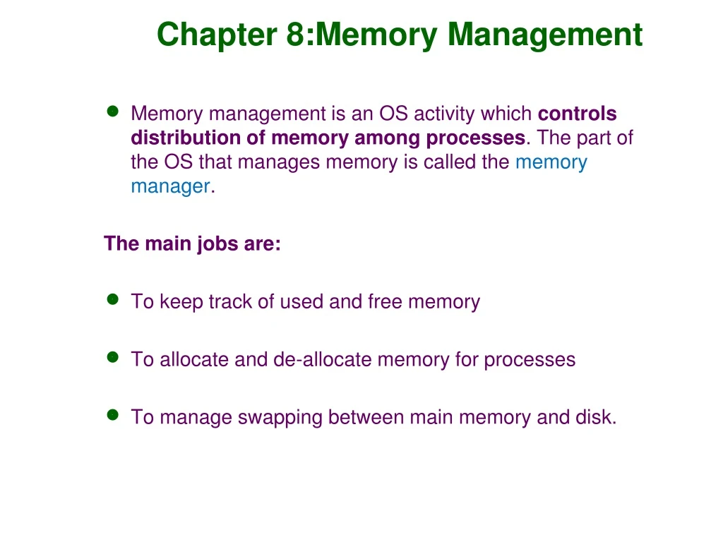
1. Chapter 8:Memory Management • Memory management is an OS activity which controls distribution of memory among processes. The part of the OS that manages memory is called the memory manager. The main jobs are: • To keep track of used and free memory • To allocate and de-allocate memory for processes • To manage swapping between main memory and disk.

2. Memory Management Memory management systems rely on the following strategies: • Memory allocation (partitioning) • Swapping • Paging • Segmentation • Virtual memory

3. Background • Memory is a large amount of words or bytes, each with its own address. The CPU fetches instructions from memory according to the value of the program counter. We are interested in only the sequence of memory addresses generated by the running program. • Program must be brought (from disk) into memory and placed within a process for it to be run • Main memory and registers are only storage CPU can access directly • Memory unit only sees a stream of addresses + read requests, or address + data and write requests • Register access in one CPU clock (or less) • Cachesits between main memory and CPU registers • Protection of memory required to ensure correct operation

4. Memory allocation Monoprogramming: • The simplest possible memory management scheme is to have just one process in memory at a time and to allow that process to use all memory. This approach is not used any more even in home computers. This approach can be as: • Device Drivers are loaded in ROM, • the rest of the OS is loaded in part of the RAM and • the user program uses the entire remaining RAM. • On computers with multiple users, monoprogramming is not used, because different users should be able to run processes simultaneously. This requires having more than one process in memory (i.e. multiprogramming), thus another approach for memory management is multiprogramming.

5. Memory allocation Multiprogramming – with fixed partitioning: • With this strategy, the memory is divided into N (typically unequal) portions called “partitions”. When a job arrives, it can be inserted into the smallest partition large enough to hold it. • Basically, we might have a single job queue served by all the partitions or one input (job) queue for each partition. multiple queues single queue

6. Memory protection • Two special registers called Base and Limit (define the logical address space) are usually used per partition for protection. • CPU must check every memory access generated in user mode to be sure it is between base and limit for that user. • Fixed partitioning method has two main problems: • How to determine the number of partitions and size of each partition? • Fragmentation (both internal and external) may occur!

7. Fragmentation • The algorithms described above suffer from external fragmentation. As processes are loaded and removed from memory, the free memory space is broken into small regions. • External fragmentation occurs when enough memory space exists to satisfy a request but it is not contiguous; storage is fragmented into a large number of small pieces. 1000 Assume that a new process P4 arrives requiring 250 bytes. Although there are 350 bytes free space, this request cannot be satisfied. This is called external fragmentation of memory. 800 600 250 100

8. Fragmentation • Assume that a new process arrives requiring 18,598 bytes. If the requested block is allocated exactly, there will be a hole of 2 bytes. The memory space required to keep this hole in the table used for indicating the available and used regions of memory will be larger than the hole itself. • The general approach is to allocate very small holes as a part of larger request. The difference between the allocated and requested memory space is called internal fragmentation - memory that is internal to a partition, but is not being used. a hole of 18,600 bytes a hole of 18,600 bytes External Fragmentation– total memory space exists to satisfy a request, but it is not contiguous Internal Fragmentation– allocated memory may be slightly larger than requested memory; this size difference is memory internal to a partition, but not being used

9. Compaction • One possible solution to external fragmentation problem is compaction. • The main aim is to shuffle the memory contents to place all free memory together in one block. 1000 1000 800 650 600 450 250 100 100 50 50

10. Memory allocation Multiprogramming – with variable partitioning: • In this method, we keep a table indicating used/free areas in memory. Initially, whole memory is free and it is considered as one large block. • When a new process arrives, we search for a block of free memory, large enough for that process. • The number, location and size of the partitions vary dynamically as process come and go. • The memory usually divided into two partitions: one for the resident operating system and one for the user processes. We can place the operating system in either low memory or high memory.

11. Variable partitioning - example A is moved into main memory, then process B, then process C, then A terminates or is swapped out, then D comes in, then B goes out, then E comes in. If a block is freed, we try to merge it with its neighbors if they are also free.

12. Selection of blocks There are three main algorithms for searching the list of free blocks for a specific amount of memory: • First-Fit:Allocate the first free block that is large enough for the new process (very fast). • Best-Fit:Allocate the smallest block among those that are large enough for the new process. We have to search the entire list. However, this algorithm produces the smallest left-over block. • Worst-Fit:Allocate the largest block among those that are large enough for the new process. Again, we have to search the list. This algorithm produces the largest left-over block.

13. Example Consider the example given on the right. Now, assume that P4 = 3K arrives. The block that is going to be selected depends on the algorithm used.

14. Example before insertion Exercise: What will be the resulting memory map if the folliwing processes arrive in order P5=10K, P6=9K, P7=1K and P8=5K?

15. Relative performance • Simulation studies show that Worst-fit is the worst and in some cases, First-fit has better performance than Best-fit. • Generally, variable partitioning results in better memory utilization than fixed partitioning; causes lesser fragmentation; and serves large or small all partitions equally well.

16. Swapping • In a time sharing system, there are more users than there is memory to hold all their processes. → Some excess processes which are blocked must be kept on backing store. Moving processes between main memory and backing store is called swapping. • A process can be swapped temporarily out of memory to a backing store, and then brought back into memory for continued execution. • Backing store – fast disk, it must be large enough to accommodate copies of all memory images for all users; • The main problem with swapping and variable partitions is to keep track of memory usage. Some techniques to address this issue are: • Bit Maps • Linked lists • Buddy system.

17. Schematic View of Swapping

18. Bit Maps Technique • With a bit map, memory is divided up into allocation units (8-512 bytes). Corresponding to each allocation unit is a bit in the bit map, which is 0 if the unit is free and 1 if it is occupied The main problem with bit maps is searching for consecutive 0 bits in the map for a process. Such a search takes a long time.

19. Linked lists Technique • The idea is to maintain a linked list of allocated and free memory segments, where a segment is either a process or a hole between two processes. Each entry in the list specifies a hole (H) or process (P), the address at which it starts, the length and a pointer to the next entry. The main advantage of this is that the list can be easily modified when a process is swapped out or terminates.

20. Example • Consider the previous system, and assume process C is swapped out. H

21. A new process is added To allocate memory for a newly created or swapped in process, First-fit or Best-fit algorithms can be used:

22. A new process is added

23. Buddy system technique • With this technique, the memory manager maintains a list of free blocks of size as power of two (i.e. 1, 2, 4, 8, 16, 32, 64, …, maxsize). • For allocation, the smallest power of 2 size block that is able to hold the process is determined. If no block with such size is available then immediately the bigger free block is split into 2 blocks (called buddy blocks), …. • This buddy system is very fast, but it has the problem of fragmentation.

24. Example - initially one hole of 1024 KB

25. Paging • A memory management scheme that avoids external fragmentation and the need for compaction. • Paging is implemented through cooperation between the operating system and the computer harfware. • Paging permits a program to be allocated noncontiguous blocks of memory (physical address space of a process can be noncontiguous). • Divide physical memory into fixed-sized blocks called frames (size is power of 2). • Divide logical memory and programs into blocks of same size called pages. • Keep track of all free frames. • To run a program of size N pages, need to find N free frames and load program. • Set up a page table to translate logical to physical addresses. • Still have Internal fragmentation

26. Logical Address Concept • Remember that the location of instructions and data of a program are not fixed. • The locations may change due to swapping, compaction, etc. • To solve this process, a logical address is introduced. • A logical address is a reference to a memory location independent of the current assignment of data in memory. • A physical address is an actual location in memory. • Logical address– generated by the CPU; also referred to as virtual address • Physical address– address seen by the memory unit • Logical address space is the set of all logical addresses generated by a program • Physical address space is the set of all physical addresses generated by a program

27. Address Translation Scheme • Address generated by CPU is divided into: • Page number (p)– used as an index into a page table which contains base address of each page in physical memory • Page offset (d)– combined with base address to define the physical memory address that is sent to the memory unit • For given logical address space 2m and page size2n • p is an index into page table and d is the displacement within the page

28. Paging Hardware Each process has a page table.

29. Paging Model of Logical and Physical Memory

30. Paging Example: Mapping logical addresses to physical adresses • In the logical address, n=2 and m=4 • Logical adrees space, 2m = 16 bytes • Page size, 2n = 4bytes • Physical memory size = 32bytes • # of frames = phys. memory size/page size • 32/4 = 8 frames • For a 32-bytes memory with 4-bytes pages consider the following mapping. Logical address 0 is page 0, offset 0. Indexing into the page table, we find that page 0 in frame 5. Thus, logical address 0 maps to physical address 20(=(5x4)+0). Logical address 3(page 0, offset 3) maps to physical address 23(=(5x4)+3). Logical address 4 is page 1, offset 0 is mapped to frame 6. Logical address 4 maps to physical address 24(=(6x4)+0) Logical address 13 (page 3, offset 1) maps to physical address 9(=(2x4)+1)

31. Free Frames Before allocation After allocation

32. Free Frames • When a new process formed of Npages arrives, it requires N frames in the memory. • We check the free frame list. If there are more than or equal to Nfree frames, we allocate N of them to this new process and put it into memory. • We also prepare its page table, since each process has its own page table. However, if there are less than N free frames, the new process must wait. Operating System Concepts

33. Paging Example S = page size p = [logical address div S], and d = [logical address mod S] (i.e. d is the position of a word inside the page). Let S (page size) = 8 words (2n= 23 → d is represented by 3 bits) Let physical memory size = 128 words. frame size = page size = 8 words no. of frames = physical memory size / frame size = 128 / 8 = 16 8 → 23 , d (offset) 3 bits, 16→ 24 , f (frame ) 4 bits. Page indices in a 3- pages program 0, 1, 2 (in binary 00, 01, 10) with 8 words in each (see next slide).

34. Paging Example: A 3-pages program

35. Implementation of Page Table • Every access to memory should go through the page table. Therefore, it must be implemented in an efficient way. Use fast dedicated registers (page table registers) • CPU dispatcher loads(stores) fast dedicated registers as it loads(stores) other registers. Only the OS should be able to modify these registers. • If the page table is large(for example 1 million entries), this method becomes very inefficient.

36. Implementation of Page Table Keep the page table in main memory • Here, a page table base register (PTBR) is needed to point to the first entry of the page table in memory. • This is a time consuming method, because for every logical memory reference, two memory accesses are required(one for page table entry, and one for the data / instruction • Use PTBR to find page table, and accessing the appropriate entry of the page table, find the frame number corresponding to the page number in the logical address, • Access the memory word in that frame.

37. Implementation of Page Table Use associative registers (special fast-lookup cache memory) • These are small, high speed registers built in a special way so that they permit an associative search over their contents (i.e. all registers may be searched in one machine cycle simultaneously.) • Associative registers are quite expensive. So, we use a small number of them. • When a logical memory reference is made: • Search for the corresponding page number in associative registers. • If that page number is found in one associative register: • Get the corresponding frame number, • Access the memory word. • If that page number is not in any associative register: • Access the page table to find the frame number, • Access the memory word → (Two memory access). • Also add that page number – frame number pair to an associative register, so that they will be found quickly on the next reference.

38. Associative Memory • Associative memory – parallel search • Address translation (p, d) • If p is in associative register, get frame # out • Otherwise get frame # from page table in memory

39. Paging Hardware With TLB An associative memory also called translation look-aside buffers (TLBs).

40. Hit Ratio • The hit ratio is defined as the percentage of times that a page number is found in the associative registers; ratio related to number of associative registers • With only 8 to 16 associative registers, a hit ratio higher than 80% can be achieved. EXAMPLE: • Assume we have a paging system which uses associative registers with a hit ratio of 90%. Assume associative registers have an access time of 30 nanoseconds, and the memory access time is 470 nanoseconds. Find the effective memory access time (emat) Case 1: The referenced page number is in associative registers: → Effective access time = 30 + 470 = 500 ns. Case 2: The page number is not found in associative registers: → Effective access time = 30 + 470 + 470 = 970 ns.

41. Hit Ratio • Then the effective memory access time can be calculated as follows: emat = 0.90 * 500 + 0.10 * 970 = 450 + 97=547ns. So, on the average, there is a 547-470=77 ns slowdown

42. Segmentation systems • Segmentation is a memory-management scheme that supports user view of memory. • A program is a collection of segments. A segment is a logical unit such as: main program, procedure, function, method, object, local variables, global variables, common block, stack, symbol table, arrays

43. Segmentation • In segmentation, programs are divided into variable size segments. • Each segment has a name and length. • Every logical address is formed of a segment number and an offset within that segment. • Programs are segmented automatically by the compiler.

44. User’s View of a Program

45. Logical View of Segmentation 1 4 2 3 1 2 3 4 user space physical memory space

46. Segmentation Architecture • Logical address consists of a two tuple: <segment-number, offset>, • Segment table– maps two-dimensional physical addresses; each table entry has: • base– contains the starting physical address where the segments reside in memory • limit– specifies the length of the segment • For logical to physical address mapping, a segment table (ST) is used. When a logical address <segment -numbr,d> is generated by the processor: • Check if ( 0 ≤ d < limit ) in ST. • If o.k., then the physical address is calculated as Base + d, and the physical memory is accessed at memory word ( Base + d ).

47. Segmentation Hardware

48. Example of Segmentation

49. Example of Segmentation • For example, assume the logical address generated is <1,123> • Check ST entry for segment #1. The limit for segment #1 is 400. Since 123<400,we carry on. • The physical address is calculated as: 9300 + 123 = 9423, and the memory word 9423 is accessed.

50. Sharing of Segments Sharing text editor among users Sharing functions among programs