Download
1 / 40
400 likes | 519 Views
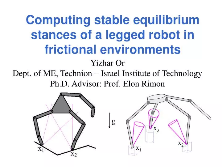
Computing stable equilibrium stances of a legged robot in frictional environments. Yizhar Or Dept. of ME, Technion – Israel Institute of Technology Ph.D. Advisor: Prof. Elon Rimon. g. x 3. x 2. x 1. Outline. 2D:. Computation of frictional equilibrium stances

E N D
Computing stable equilibrium stances of a legged robot in frictional environments Yizhar Or Dept. of ME, Technion – Israel Institute of Technology Ph.D. Advisor: Prof. Elon Rimon g x3 x2 x1
Outline 2D: • Computation of frictional equilibrium stances • Robustness w.r.t disturbance forces and torques • Dynamics – contact modes and strong stability 3D: • The support polygon principle for flat terrains • Geometric Parametrization of equilibrium forces in 3D • Exact Computation of frictional equilibrium stances • Polyhedral approximation of equilibrium stances
g Problem Statement Setup: mechanism modeled as a variable c.o.m. body Given a 2D (3D) multi-limbed mechanism standing on a terrain with k frictional contacts, where should the center-of-mass be for: • Static equilibrium? • Robustness w.r.t disturbance forces? • Dynamic stability?
Applications • Quasistatic legged locomotion on rough terrain • (spider robots, snake robots, climbing, search-and-rescue robots) • Graspless manipulation (part feeding, assemblies) • Motion planning for Hybrid wheeled-legged robots • Semi-dynamic locomotion
Application - Three-Legged Locomotion 2-3-2 gait pattern: • Select 2-contact postures that share a common contact point • 3-contact stage connecting two consequent 2-contact postures • At the 3-contact stage: straight line motion of center-of-mass
Related Work – 2D • Mason, Rimon, Burdick (1995): Frictionless postures under gravity • Greenfield, Choset and Rizzi (2005): planning quasistatic climbing via bracing • Mason (1991): Graphical methods for frictional equilibrium in 2D • Erdmann (1998): Two-palm manipulation with friction in 2D • Lotstedt (1982); Erdmann (1984); Mason & Wang (1988); Rajan, Burridge and Schwartz (1987); Dupont (1992): Contact modes and frictional dynamic ambiguity • Trinkle & Pang (1998): Strong stability, LCP formulation of frictional dynamics
Related Work – 3D • McGhee and Frank, 1968: The support polygon principle for legged locomotion • Bretl, Latombe (2003): PRM-based motion planning algorithm for climbing on vertical walls with discrete supports • Mason, Rimon and Burdick , 1997: Computing stable equilibrium frictionless stances in 3D • Han, Trinkle and Li, 2000: Feasibility test of frictional postures in 3D as LMI problem • Bretl and Lall, 2006: Adaptive polyhedral approximation of 3D equilibrium stances
Equilibrium condition: • where t(x)= xJfext+text x Statics in 2D - LP Formulation • Center of mass:x2 • External wrench:w=(fext,text) 2 • Contact forces:f2k • Friction Cones Bounds: Bf ≥ 0
tmin = min{-Gtf} tmax = min{-Gtf} s.t. s.t. Gff=-fext Bf ≥ 0 Gff=-fext Bf ≥ 0 Statics - LP Formulation (cont’d) Theorem: The feasible k-contact equilibrium region: R(w) = {x: tmin xJfext + texttmax} where Infinite strip parallel to fext
R(wo) g x 2 x 1 Two Contacts Graphical Example wo=(fg,0) m = 0.3
R(wo) g x 2 x 1 Two Contacts Graphical Example (cont’d) m = 2.0
S++ = Strip (C1+,C2+) S--= Strip (C1-,C2-) + - + + S S S-+ = Strip (C1-,C2+) S+-= Strip (C1+,C2-) P Theorem: R(wo)= [(S++ S--) P] [(S+- S-+) P ] R(wo) _ 2 Contacts - Graphical Characterization x 2 P = Strip (x1, x2) x 1
R(wo) R R g 56 13 Algorithm: k-Contacts - Graphical Characterization R(w) = =conv{Rij (w) } x x 1 x x x 4 6 x 5 3 2
g b fext c.o.m. dx • Robust Equilibrium Region:R(N) = R(w) wN External Wrench Neighborhood • Wrench magnitude scales static response • Parametrize wext=(fx,fy,text): • External wrench neighborhood: • N = {(p,q): -k≤p≤k , -n≤q≤n}
R(N) = R(w) fext wN fext n Then R(N) =R(wi) fg i x 2 x 1 Robust Equilibrium Region – Example Recipe: If N = conv {wi} R(N)
3 equations 3+2k unknowns Dynamic Contact Modes Theory ma = fext + f1 + f2 + …+ fk Ica = text + (x1-x)×f1 +… (xk-x) ×fk Contact modes (F, R, U, W) (or S) • Contact modes add 2k equations a unique dynamic solution as a function of x • Contact Mode’s inequalities Feasibility Region of x
g Example of Dynamic Ambiguity Contact mode UF:
The Strong Stability Criterion Strong Stability (Trinkle and Pang, 1998): S (w) = RSS(w) - RFF (w) RUF (w) ... RWW(w) • Eliminates ambiguity – only static solution is feasible • Any roll/slide/break motion cannot evolve (at zero velocity) • Yet, not formally related to classical dynamic stability • (bounded response to bounded position/velocity perturbations) • Does not always imply bounds on c.o.m. height Must be augmented with robustness
Robust Stability:S(N) = S(w) wN Define: Robust Equilibrium Region: RSS(N) = RSS(w) wN RXY(N) = RXY(w) Non-Static Modes’ N-Feasible Region: wN Robust Stability Region: S(N) = RSS(N) -RFF(N) RUF(N) ... RWW(N) Robust Stability - Definitions Strong Stability: S (w) = RSS(w) - RFF (w) RUF (w) ... RWW(w)
Definition:RXY(N) = RXY(w) wN Non-Static Modes N-Feasible Region • Express RXY as an intersection of halfspaces • in a four-dimensional space: Fi(x,y,p,q) ≥ 0 • RXY(N) is the projection of RXY onto xy plane The Silhouette Theorem: The Silhouette curves of the projection are critical values of the projection function, on which the generalized normal of RXY is parallel to xy plane.
N N-Feasible Region of UF Mode • Critical curves fi(x,y,p,q) are • linear in p,q and quadratic in x,y • Critical curves generate • cell arrangement in xy plane • Line-Sweep Algorithm: • identifies the cells and generates sample points • Checking cell membership: LP problem in p,q
N N N S(N) N S(N) S(N) S(N) Example - Robust Stability Region S(N) = RSS(N) - RFF(N) RUF(N) ... RWW(N) r=0.05 r=0.1 r=0.25
Strong Stability and Dynamic stability Force Closure asymp. stability under keep-contact perturbations Here: no force closure, passive contacts, arbitrary perturbations Two contacts - neutralstability under keep-contact perturbations Strong Stability non-static modedecays until collision • How to model collisions? treat sequence of collisions? • Does strong stability really leads to dynamic stability? • How to design stabilizing joints’ control laws • for a legged robot?
Frictional Equilibrium Stances in 3D • Analyze 3D equilibrium stances of legged mechanisms in frictional environments • Support Polygon criterion does not apply for non-flat terrains • Exact formulation of equilibrium region • Efficient conservative approximation by projection of convex polytopes g
Problem Statement • Characterize feasible equilibrium postures of a multi-limbed mechanism supported against frictional environment in 3D. • Given k frictional contacts, find the feasible region R of center-of-mass locations achieving frictional equilibrium. • Assumption: point contacts, uniform friction coefficient m. • Friction Cones in 3D: Ci = {fi : (fi⋅ni)≥0and(fi⋅si)2 + (fi⋅ti)2≤m2(fi⋅ni)2} • Feasible equilibrium region in 3D:
R is a vertical prism with horizontal cross-section . Focus on computing the boundary of for 3-contact stances. Basic Properties of R • R is a convex and connected set. • The dimension of R is generically min{k,3}. Assumption: upward pointing contacts: fie > 0 for all fi Ci, where e is the upward direction
Motivational Example m = 0.5 R g z x y The Support Polygon Principle: x must lie in the vertical prism spanned by the contacts:
X3 y ??? X2 X1 x x Motivational Example (cont’d) top view m = 0.2 g z x3 x2 y x1 Support Polygon Principle is unsafe!!!
Parametrizing Equilibrium Forces • Horizontal and vertical components: • fi must intersect a common vertical line lr
Permissible Polygonal Region of r • Projected frictional constraints: • rmust lie in the polygonal regionP = P+ P- ,where
y P+ P- x Graphical Example of P top view
p2 p3 p1 where Complete Graphical Parametrization • Action line of fi intersects the common vertical line lr at pi • Define zi – height of pi about xi zi = e∙(pi –xi) • Parametrize contact forces by (r,z) 2 3, where z=(z1,z2,z3):
P and Q = Q1 Q2 Q3 Qi where Ci P Permissible Region in (r,z) space • The permissible region: (r,z) Q = Q1 Q2 Q3 , where • for fi lying on the boundary of Ci ,zi=zi*(r)
Computing the Boundary of • Torque balance implies a map from (r,z) to : Horizontal cross section is the image of Q under • Formulate the restriction of to all possible manifolds of Q • Compute critical curves of on each manifold of Q • Candidate boundary curves of are -image of critical curves
type-2 boundary fiCi,fjCj, r=r* type-3 boundary fi Ci, i=1..3 type-1 boundary fi,fj≠0 ; fk=0 Graphical Example of y x
Conservative Polyhedral Approximation • Replacing exact friction cones with inscribed pyramids. • Reduces to projection of a convex polytope onto a plane • Approximate outer bound by taking circumscribing pyramids • Graphical example – with 6-sided pyramids
x 3 y x x 2 1 x Polyhedral Approximation of R - Example top view
Already done In progress Future Research • Physical geometric intuition of boundary curves, effect of m • Relation to line geometry and parallel robots’ singularities • Generalization to multiple contact points • Robustness with respect to disturbance forces and torques • Elimination of non-static contact modes • (Complementarity formulation, Pang and Trinkle, 2000) • Application to legged locomotion on rough terrain in 3D
g x3 x2 x1 Computing stable equilibrium stances of a legged robot in frictional environments Yizhar Or Dept. of ME, Technion – Israel Institute of Technology Ph.D. Advisor: Prof. Elon Rimon izi@technion.ac.il robots.technion.ac.il/yizhar
Thank You תודה רבה