Download
1 / 19
190 likes | 218 Views
Explore the GALS method for space-time reconstruction and analysis using least squares. Learn about error estimates, real data applications, and potential prospects in physics research.

E N D
G A L S Gradient Analysis with Least Squares M. Hamrin, K. Rönnmark, and J. Vedin Department of Physics, Umeå University SE-901 87 Umeå, Sweden
Outline • Basics: GALS method • Basics: numerical routine • Error estimates • GALS applied on test data • GALS with real Cluster data • Summary and prospects Hamrin et al., Bucharest, Sep. 2005
rr For every sampled time there are 5 unknown: f, and 4 known variables (4 sc): f1,f2,f3, f4 N sampled times: Overdetermined system with 4N knowns. With a least squares method the higher order terms (H.O.) are minimized. 1. Basics: GALS method rsc sc positions in time and space (t,x,y,z) fsc scalar field (e.g. Bx) sampled by sc1…4 rr space-time reconstruction point fr reconstructed field at rr □·frreconstructed time and space gradients Taylor expanding → fsc = fr + (rsc– rr) □·fr + H.O. Hamrin et al., Bucharest, Sep. 2005
Rewriting: where . The RHS is dominated by distant points, i.e. (rsc– rr)=Δsc large, but dividing the importance of higher derivatives is reduced when Δsc>λ. 2. Basics: numerical routine Hamrin et al., Bucharest, Sep. 2005
GALS determines fr and □·fr by minimizing: using the standard MATLAB routine lscov We generalize by using: 2. Basics: numerical routine Advanced users: align κ with the current sheet. Hamrin et al., Bucharest, Sep. 2005
3. Error estimates It should be possible to obtain reasonable error estimates. We are working on it… Hamrin et al., Bucharest, Sep. 2005
The CS becomes somewhat smoothed. Artificial Jz due to . A (small) due to . Artificial time variation . Hamrin et al., Bucharest, Sep. 2005 4. GALS applied on test data 1. • Infinite Gauss.current sheet (CS) in xy plane. • Equilateral ”Cluster” tetrahedron (E=P=0). • CS width W=20km. • ”Cluster” charac. size L=200km. • Sc velocity perp. to current sheet.
Hamrin et al., Bucharest, Sep. 2005 4. GALS applied on test data 1. • GALS better than Curlometer localizing CS. • Artifizial Jz. • Pronounced bipolarity in Jz for Curlometer.
Hamrin et al., Bucharest, Sep. 2005 4. GALS applied on test data 2. • Cigar shaped sc configuration flying 45° toward the CS.
Hamrin et al., Bucharest, Sep. 2005 4. GALS applied on test data 2. • GALS: better localizing CS. • GALS: less bi-polarity.
Hamrin et al., Bucharest, Sep. 2005 4. GALS applied on test data 3. • Cigar shaped sc configuration flying 45° toward the CS.
Hamrin et al., Bucharest, Sep. 2005 4. GALS applied on test data 3. • GALS and Curlometer comparable. • Bi-polarity very small.
Hamrin et al., Bucharest, Sep. 2005 5. GALS with real Cluster data 1. • Magnetopause crossing with thin CS. • Carefully selected κ aligned with CS. • Magnetopause nicely reconstructed. • Data gets automatically smoothed by GALS.
GALS Curlometer Jy 1 sc method Hamrin et al., Bucharest, Sep. 2005 5. GALS with real Cluster data 1. • GALS resolves CS better than Curlometer. • GALS and single sc method consistent.
Hamrin et al., Bucharest, Sep. 2005 5. GALS with real Cluster data 2. • Cluster data with strangely sloping current. • Is this caused by dipole magnetic field?
Hamrin et al., Bucharest, Sep. 2005 5. GALS with real Cluster data 2. • Simulated dipole magnetic field. • The artificial current is tiny, especially for GALS.
--- GALS --- • Uses the fact that each SC samples a long time-series of, e.g., B fields. • Obtains space and time derivatives. • Current from . • Various test runs: GALS is comparable or better (!) than the Curlometer. • Not very sensitive to the satellite configuration. • It should be possible to obtain reasonable error estimates. • Possibilities for advanced users to optimize (κ, rotation) the method. 6. Summary Hamrin et al., Bucharest, Sep. 2005
6. Prospects • Error estimates. • More tests of the method on both simulated and real data. • Investigate the capacity to separate time and space variations. • Apply the method to other physical fields. Hamrin et al., Bucharest, Sep. 2005
The End Hamrin et al., Bucharest, Sep. 2005