Download
1 / 21
210 likes | 315 Views
Particle Filtering. Sensors and Uncertainty. Real world sensors are noisy and suffer from missing data (e.g., occlusions, GPS blackouts) Use sensor models to estimate ground truth, unobserved variables, make forecasts. X 0. X 1. X 2. X 3. Hidden Markov Model.

E N D
Sensors and Uncertainty • Real world sensors are noisy and suffer from missing data (e.g., occlusions, GPS blackouts) • Use sensor models to estimate ground truth, unobserved variables, make forecasts
X0 X1 X2 X3 Hidden Markov Model • Use observations to get a better idea of where the robot is at time t Hidden state variables Observed variables z1 z2 z3 Predict – observe – predict – observe…
Last Class • Kalman Filtering and its extensions • Exact Bayesian inference for Gaussian state distributions, process noise, observation noise • What about more general distributions? • Key representational issue • How to represent and perform calculations on probability distributions?
Particle Filtering (aka Sequential Monte Carlo) • Represent distributions as a set of particles • Applicable to non-gaussian high-D distributions • Convenient implementations • Widely used in vision, robotics
Simultaneous Localization and Mapping (SLAM) • Mobile robots • Odometry • Locally accurate • Drifts significantly over time • Vision/ladar/sonar • Inaccurate locally • Global reference frame • Combine the two • State: (robot pose, map) • Observations: (sensor input)
General problem • xt ~ Bel(xt) (arbitrary p.d.f.) • xt+1 = f(xt,u,ep) • zt+1 = g(xt+1,eo) • ep ~ arbitrary p.d.f., eo ~ arbitrary p.d.f. Process noise Observation noise
Particle Representation • Bel(xt) = {(wk,xk), k=1,…,n} • wk are weights, xk are state hypotheses • Weights sum to 1 • Approximates the underlying distribution
Monte Carlo Integration • If P(x) ≈ Bel(x) = {(wk,xk), k=1,…,N} • EP[f(x)] = integral[ f(x)P(x)dx ] ≈ Skwkf(xk) • What might you want to compute? • Mean: set f(x) = x • Variance: f(x) = x2 (recover Var(x) = E[x2]-E[x]2) • P(y): set f(x) = P(y|x) • Because P(y) = integral[ P(y|x)P(x)dx ]
Recovering the Distribution • Kernel density estimation • P(x) = Sk wk K(x,xk) • K(x,xk) is the kernel function • Better approximation as # particles, kernel sharpness increases
Filtering Steps • Predict • Compute Bel’(xt+1): distribution of xt+1 using dynamics model alone • Update • Compute a representation of P(xt+1|zt+1) via likelihood weighting for each particle in Bel’(xt+1) • Resample to produce Bel(xt+1) for next step
Predict Step • Given input particles Bel(xt) • Distribution of xt+1=f(xt,ut,e) determined by sampling e from its distribution and then propagating individual particles • Gives Bel’(xt+1)
Update Step • Goal: compute a representation of P(xt+1 | zt+1) given Bel’(xt+1), zt+1 • P(xt+1 | zt+1) = a P(zt+1 | xt+1) P(xt+1) • P(xt+1) = Bel’(xt+1) (given) • Each state hypothesis xk Bel’(xt+1) is reweighted by P(zt+1 | xt+1) • Likelihood weighting: • wkwkP(zt+1|xt+1=xk) • Then renormalize to 1
Update Step • wk wk’ * P(zt+1 | xt+1=xk) • 1D example: • g(x,eo) = h(x) + eo • eo ~ N(m,s) • P(zt+1 | xt+1=xk) = C exp(- (h(x)-zt+1)2 / 2s2) • In general, distribution can be calibrated using experimental data
Resampling • Likelihood weighted particles may no longer represent the distribution efficiently • Importance resampling: sample new particles proportionally to weight
Sampling Importance Resampling (SIR) variant Predict Update Resample
Particle Filtering Issues • Variance • Std. dev. of a quantity (e.g., mean) computed as a function of the particle representation ~ 1/sqrt(N) • Loss of particle diversity • Resampling will likely drop particles with low likelihood • They may turn out to be useful hypotheses in the future
Other Resampling Variants • Selective resampling • Keep weights, only resample when # of “effective particles” < threshold • Stratified resampling • Reduce variance using quasi-random sampling • Optimization • Explicitly choose particles to minimize deviance from posterior • …
Storing more information with same # of particles • Unscented Particle Filter • Each particle represents a local gaussian, maintains a local covariance matrix • Combination of particle filter + Kalman filter • Rao-Blackwellized Particle Filter • State (x1,x2) • Particle contains hypothesis of x1, analytical distribution over x2 • Reduces variance
Recap • Bayesian mechanisms for state estimation are well understood • Representation challenge • Methods: • Kalman filters: highly efficient closed-form solution for Gaussian distributions • Particle filters: approximate filtering for high-D, non-Gaussian distributions • Implementation challenges for different domains (localization, mapping, SLAM, tracking)