Dynamic Bayesian Networks and Particle Filtering

1. Dynamic Bayesian Networks and Particle Filtering COMPSCI 276 (chapter 15, Russel and Norvig) 2007

7. Dynamic Belief Networks (DBNs) Transition arcs Xt Xt+1 Yt Yt+1 Bayesian Network at time t Bayesian Network at time t+1 X10 X0 X1 X2 Y10 Y0 Y1 Y2 Unrolled DBN for t=0 to t=10

8. Dynamic Belief Networks (DBNs) Interaction graph Two-stage influence diagram

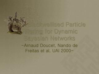
9. Notation t=0 t=1 t=2 t=1 t=2 X0 X1 X2 Xt Xt+1 Xt – value of X at time t X 0:t ={X0,X1,…,Xt}– vector of values of X Yt – evidence at time t Y 0:t = {Y0,Y1,…,Yt} Y0 Y1 Y2 Yt Yt+1 DBN 2-time slice

10. Inference is hard, need approximation Mini-bucket? Sampling?

13. Particle Filtering (PF) • = “condensation” • = “sequential Monte Carlo” • = “survival of the fittest” • PF can treat any type of probability distribution, non-linearity, and non-stationarity; • PF are powerful sampling based inference/learning algorithms for DBNs.

15. Particle Filtering

19. Example Particlet={at,bt,ct}

20. PF Sampling Particle (t) ={at,bt,ct} Compute particle (t+1): Sample bt+1, from P(b|at,ct) Sample at+1, from P(a|bt+1,ct) Sample ct+1, from P(c|bt+1,at+1) Weight particle wt+1 If weight is too small, discard Otherwise, multiply

21. Drawback of PF • Drawback of PF • Inefficient in high-dimensional spaces (Variance becomes so large) • Solution • Rao-Balckwellisation, that is, sample a subset of the variables allowing the remainder to be integrated out exactly. The resulting estimates can be shown to have lower variance. • Rao-Blackwell Theorem

22. Example Sample Only Bt