Download
1 / 19
200 likes | 326 Views
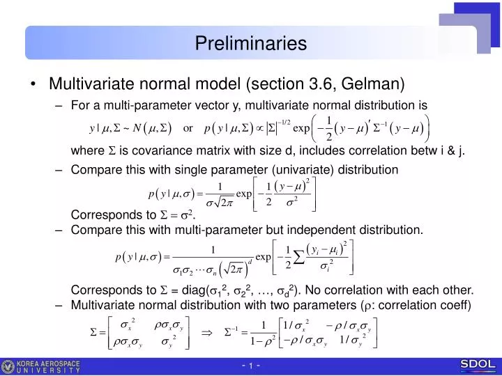
Preliminaries. Multivariate normal model (section 3.6, Gelman ) For a multi-parameter vector y, multivariate normal distribution is where S is covariance matrix with size d, includes correlation betw i & j.

E N D
Preliminaries • Multivariate normal model (section 3.6, Gelman) • For a multi-parameter vector y, multivariate normal distribution is where S is covariance matrix with size d, includes correlation betwi & j. • Compare this with single parameter (univariate) distributionCorresponds to S = s2. • Compare this with multi-parameter but independent distribution.Corresponds to S = diag(s12, s22, …, sd2). No correlation with each other. • Multivariate normal distribution with two parameters (r: correlation coeff)
Preliminaries • Multivariate normal model example • Two random variables x=[x1, x2] following multivariate normal distribution with zero means, unit variance and correlation r. • Simulate x by drawing samples with N=1000. • When there is no correlation, i.e., r=0, it is the same as sampling x1 and x2 independently, and just pair them. • As the correlation is stronger, we get the following trend. If x1 is high, x2 is also likely to be high. Independent or r=0.01 r=0.5 r=0.9 r=1.0
Correlated regression • Departures from ordinary linear regression • Previously, there were a number of assumptions.Linearity of response w.r.t. the explanatory variables Normality of the error termsIndependent (uncorrelated) observations with equal variance • Non of which is true in practice. • Correlations • Consider error between data and regression.Sometimes, error can’t be -1 at a point, +1 at the next. The change should be gradual. In this sense, errors at two adjacent points can be correlated. • If we ignore this, the posterior inference may lead to wrong result.Furthermore, prediction for future will also be wrong.
Classical regression review • Important equations • Functional form of the regression • Regression coefficients • Standard error • Coefficient of determination • Variance of coefficients • Variance of regression • Variance of prediction
Classical regression review: Bayesian version • Analytical procedure • Joint posterior pdf of b,s2 • Factorization • Marginal pdf of s2 • Conditional pdf of b • Posterior prediction version 1 Posterior prediction version 2
Correlated regression • Likelihood of correlated regression model • Consider n number of observed data y at x, where the errors are correlated. Then the likelihood of y is given bywhere S is covariance matrix with the size n. • Compare this with classical regressionwhere S = s2I, i.e., diagonal matrix with variance.
Bayesian correlated regression • Covariance matrix • We often consider variance matrix S in the following form, where Q represents correlation structure, while s2 accounts for global variance.In the matrix Q, d is a factor that controls degree of correlation. • Let’s see the behavior of function Q = exp{ -(x/d)2 } • Let’s see the behavior of correlation matrix Q (11x11) over x=0:0.1:1. • If d is small, function is narrow, correlation is small, data are independent . • If d is large, function is wide, correlation is strong. d=0.01 d=0.2 d=5
Bayesian correlated regression • Correlated y example • y ~ multivariate normal dist. with zero mean & covariance Q over x=(0,1). • Simulate y(x) over x = 0:0.1:1 with N=4, which follows multivariate normal distribution. • When there is no correlation, y(x) at adjacent x is independent each other. • As the correlation is stronger, we get the following trend. Independent or d=0.01 d=0.2 d=0.5 d=5 d=100
Bayesian correlated regression • Likelihood by QR decomposition • The likelihood is given by • Let S-1/2 be Cholesky factor (upper triangular) of S-1. Then S-1=(S-1/2)´(S-1/2). • Transform y into . Then we obtain • Comparing with classical case, we can find y, X of classical regression is replaced by & s2=1in the correlated regression.
Bayesian correlated regression • Posterior distribution • Replace by in the results of classical regression. • Joint posterior pdf of b,s2 • Factorization • Marginal pdf of s2 • Conditional pdf of b • Sampling method based on factorization approach • Draw random s2 from inverse- c2 distribution. • Draw random b from conditional pdfb|s2, which is multivariate normal.
Bayesian correlated regression • Sampling of posterior distribution by factorization • Data • Samples of 3 parameters (b1,b2 & s2) are drawn with N=5000 using the factorization approach. y=[0.95, 1.08, 1.28, 1.23, 1.42, 1.45]'; x=[0 0.2 0.4 0.6 0.8 1.0]'; posterior distribution of b1 & b2 posterior distribution of s2
Bayesian correlated regression • Posterior prediction • Case with correlation is more complicated. • Because the prediction at a new point is correlated with existing data y, we have to consider existing y as well. • For example, if we wish to predict height of a new child whose brothers already exist as old data, we should account for these in the prediction. • Consider a new point to get predicted . Joint distribution of existing set y and new single is given by multivariate normal distribution: • Using the properties of MVN, conditional distribution of on y is obtained, which is the MVN with the mean and variances: where .
Bayesian correlated regression • Posterior prediction • Once we have samples of b, s2 at hand, we can proceed to obtain posterior prediction at an arbitrary using following equations. • Using every individual sample set (b, s2), calculate E & var. • Then draw random sample of that follows MVN with E & var. • Over the range x=(0,1) with the interval 0.05, samples of posterior predictive distribution is obtained. d=0.01 d=0.1 d=0.5 Classical regression
Discussions on the posterior prediction • Interpolation: • At every observation point, any realization of predicted y always interpolates the data y. The variance at the data point also vanishes. • The reason is explained in the following.
Discussions on the posterior prediction • Choice of correlation factor • The distribution shape largely depends on the value of d. • For small d, which is small correlation, y(x) at adjacent x independent each other, which leads to the result closer to classical regression. • For large d, strong correlation between adjacent points leads to the unique knotted smoother shape like the figure, because of still passing thru the data. d=0.01 d=0.1 d=0.5
Discussions on the posterior prediction • Choice of correlation factor • In the Bayesian inference, this d can be added as the unknowns as well. • From the joint posterior pdf, not only the samples of b, s2 but also d are obtained. • In this case, we have no other way but to use MCMC. d=0.01 d=0.1 d=0.5
Practice example • Sampling by MCMC • This will be implemented and discussed depending on the availability. • Only the results are suggested here. d unknown d=0.1 d=0.2
Kriging surrogate model • Posterior prediction • Posterior prediction is given by the MVN with the mean and variances: • Version 1: • Use sample set (b,s2) to calculate E & var. Then draw sample from MVN. • Version 2: • Use deterministic for E, while using samples s2 for var. Then draw sample from MVN. • Kriging surrogate model • Kriging model is the mean E of version 2, which is a single deterministic curve. Recall that this curve also interpolates the data.
Kriging surrogate model • Kriging surrogate model • The model is useful in Design & Analysis of Computer Experiments (DACE) because computer model has no error, exact at the data, so interpolation is better than the approximation. • The DACE has approached differently and found the same expression. • However, DACE is not interested with the uncertainty. Only the deterministic model is obtained, by applying MLE method: • Take log to this, and take partial derivative w.r.t. b,s2and . Then we get simultaneous equations. Solve them to obtain