Download
1 / 37
451 likes | 1.71k Views
Regression in geoDA. Example regression analyses for Illiteracy Rate ( ILLITERACY) ChinaData.shp (n=35) 1. Simple regression with URBAN_POP_ ChinaData_29 (n=29) 2. Simple regression with URBAN_POP 3. Multiple regression with URBAN_POP and RMB_PC_UR_

E N D
Regression in geoDA Example regression analyses for Illiteracy Rate ( ILLITERACY) ChinaData.shp (n=35) 1. Simple regression with URBAN_POP_ ChinaData_29 (n=29) 2. Simple regression with URBAN_POP 3. Multiple regression with URBAN_POP and RMB_PC_UR_ 4. Spatial lag and error multiple regression 5. Multiple regression with log of Illiteracy Briggs Henan University 2010
Running Regression in geoDA: I 1 File>Open Shape File ChinaData Tools>Weights> Open or Create Need weights to test for spatial autocorrelation. Generally, always use a weights file. You can begin with Method>Regress if --very large number of observations (over 1,000) --no spatial weights --data only in a .dbf file 2 Methods>Regress Place as below If you have a large number of observations, do not Need this for Moran’ s I for residuals
Running Regression in geoDA: II Select one dependent variable One or more independent variables Selecttype of regression: Classic or Lag or Error Warning-bug! Use Suggested name. The names are reversed here! Click OK to save these. Saves values for Predicted Y and Residuals in the table --use Table>>Promotion to see them in table. --you can map them or draw graphs --use Table >> Save to Shapefile if you want to keep them permanently Click RUN, then Click SAVE
Running Regression in geoDA: III Results are saved in this text file. It is saved in the same folder as the shapefile. You can rename it and change location. Click OK to see the results. (You can also open the file later with a program such as Notepad) --scroll to end of file since results are added to end if file already exists Warning: if you want the residuals (see previous slide) you must click Savebefore clicking OK Click Reset to run a different regression The results
Summary: Running Regression in geoDA Warning-bug! Use Suggested name. The names are reversed here! Select variables as below. Select type of regression: Classic Lag Error File>Open Shape File ChinaData Tools>Weights> Open or Create (need weights to test for spatial autocorrelation in residuals) Methods>Regress Place as below Click OK to save these. Use Table>Promotion to see them in table. Click OK in Regression window to see results --scroll to end of file since results are added to end if file exists already Click RUN, then Click SAVE
Regression for Provinces: n = 35 Briggs Henan University 2010 • Next slide shows results from running a simple regression with ChinaData.shp Y = Illiteracy rate (ILLITERACY) X = % of population urban (URBAN_POP_) • All provinces included • Note problems with • Extreme value for Xizang/Tibet • Zeros (0) for missing data on X variable (Taiwan, Macau, Hong Kong, P’eng-hu) • Solution: Reduced data set to 29 using ArcGIS • (do not know how to do this in geoDA!)
Display table: Table >PromotionPlot using: Explore >ScatterPlot Results for simple regression Note: mean of residuals is always zero Residual Variation OLS_Resid v. Urban Pop% Total Variation Illiteracy v. Urban Pop% Predicted by Regression OLS_Predict v. Urban Pop% Extreme value identified by linking: Xizang/Tibet Briggs Henan University 2010
Partitioning the Variance on Y Residual Variation OLS_Resid v. Urban Pop% Total Variation Illiteracy v. Urban Pop% Predicted by Regression OLS_Predict v. Urban Pop% Y Y Y (Y-Ỹ) Y Ỹ SS Residual or Error Sum of Squares SS Total or Total Sum of Squares SS Regression or Explained Sum of Squares Briggs Henan University 2010
Simple Regression Results from GeoDA: general Statistics for dependent variable n = 35 Not statistically significant Results for overall regression explains only 4.6% of variance in Y Sigma-square= Variance of the estimate = 1368.89/33=41.4816 SE of regression=standard error of the estimate=√41.4816=6.44062 Identical in simple regression Results for each regression coefficient Y= 11.3146 - 6.578X Briggs Henan University 2010
Simple Regression Results from GeoDA:spatial n = 35 Moran’s I for regression residuals --not statistically significant (p=.09) Space > Univariate Moran for variable: OLS_Resid Same results! Briggs Henan University 2010
Results with omitted observations:much better! Now explains 33.41% But probably non-linear Statistically significant Spatial autocorrelation not a problem Data for China Provinces 29: excludes Xizang/Tibet, Macao, Hong Kong, Hainan, Taiwan, P'eng-hu Briggs Henan University 2010
Multiple Regression Results n = 29Illiteracy with % Pop Urban and Urban Income Overall Results Results for each variable significant Not significant Spatial Results Not significant Briggs Henan University 2010
Residual Analysis:Illiteracy v. Urban Pop % and UrbanIncomePerCapita Moran’s I = .0226 p = 0.5520 Not statistically significant No Spatial autocorrelation in residuals Briggs Henan University 2010
Spatial Error Model Resultsillustrative only: not needed Spatial error not significant Briggs Henan University 2010
Spatial Lag Model Resultsillustrative only: not needed Spatial lag not significant Briggs Henan University 2010
Regression Results Summary Briggs Henan University 2010
Note on:Variables Saved for Spatial Models Again, labels are reversed. Use suggested variable names. ERR_ indicates use of Spatial Error model. LAG_indicates use of Spatial Lag Model OLS_ indicates use of classic model For the spatial lag model, there is a distinction between the residual and the prediction error. The latter is the difference between the observed value and the predicted value that uses only exogenous variables, rather than treating the spatial lag Wy as observed. (Documentation for 905i, page 53) Prediction error (xxx_PRDERR): calculated without including spatial term. Residual error (xxx_RESIDU): calculated including spatial term Briggs Henan University 2010
Table >> Add Column Table >> Field Calculator Improving the modelRelationship is Non-linearUse log of Illiteracy Briggs Henan University 2010
The same plots using ExcelRelationship is Non-linear Illiteracy Log of Illiteracy Urban pop % Briggs Henan University 2010
Y = Log of Illiteracy R2 increases from 38% to 83% ! Urban Income now significant and Urban Population is not! Briggs Henan University 2010
Log of Illiteracy:makes relationship linear Urban Income now significant, and % urban not significant. --these two variables are highly intercorrelated --see next slide Briggs Henan University 2010
Inter-Correlation between Urban Population and Urban Income R2 for Urban Pop versus Urban Income 0.84 R is .92 N=29 Urban Population Urban Income Briggs Henan University 2010
Table >> Add Column then use Table >> Field Calculator • Creating a better model • Transforming dependent and/or independent variables can often improve the predictive capability of regression models • geoDA has several capabilities to support this. Briggs Henan University 2010
Other software options for multiple regression Briggs Henan University 2010 • Multiple regression of the type discussed here is not available in ArcGIS • Only geographically weighted regression available (there is a multiple regression for raster data but it is only in ArcInfo Workstation—difficult to use) • Use geoDA to create spatial lag variables, then use standard statistical packages such as SAS, SPSS or STATA • Use R • Free open source software, but difficult to use • http://cran.r-project.org/web/views/Spatial.html • CrimeStat III has some support for spatial regression http://www.icpsr.umich.edu/NACJD/crimestat.html • For a good list of spatial software sources, go to: http://en.wikipedia.org/wiki/List_of_spatial_analysis_software
What have we learned today? Briggs Henan University 2010 • How to use geoDA to run • classic regression models • Spatial Lag models • Spatial Error Models • Importance of examining data for “problems” • Can have a very large affect on results • Missing data and zeros • Extreme values can dominate results • Using transformations to create a better model
Geographically Weighted Regression Briggs Henan University 2010
Geographically Weighted Regression • The idea of Local Indicators can also be applied to regression • Its called geographically weighted regression • It calculates a separate regression for each polygon and its neighbors, • then maps the parameters from the model, such as the regression coefficient (b) and/or its significance value • Mathematically, this is done by applying the spatial weights matrix (Wij) to the standard formulae for regression See Fotheringham, Brunsdon and Charlton Geographically Weighted Regression Wiley, 2002 Xi Briggs Henan University 2010
Problems with Geographically Weighted Regression Xi Briggs Henan University 2010 • Each regression is based on few observations • the estimates of the regression parameters (b) are unreliable • Need to use more observations than just those with shared border, but • how far out do we go? • How far out is the “local effect”? • Need strong theory to explain why the regression parameters are different at different places • Serious questions about validity of statistical inference tests since observations not independent
GWR in ARCGIS Briggs Henan University 2010 • Requires ArcInfo, Spatial Analyst or Geostat. Analyst license • Shapefile is created: • Open its table to see results • for each polygon there are standard regression results • Condition variable: indicates when the results are unstable due to local multicollinearity • Results not good if condition > 30, Null, or -1.79e+308 • Use source_ID to join with FID of original data to identify observations
Usage Tips from ArcGIS Help Briggs Henan University 2010 • Use projected data • Observations included in each regression depend on kernal type, bandwidth method and bandwidth distance parameters set by user • Max of 1,000 observations in any one local regression • Multicollinearity can be a problem • if variables cluster spatially • if use binary/nominal/categorical variables • Never use dummy variables (1/0) to index spatial regions • (Multicollinearity: intercorrelation between independent variables) • Not appropriate for small data sets: need several hundred observations • Shapefiles cannot store “nul l” values: treated as zero. Be sure there is no missing data
Running GWR in ArcGIS Briggs Henan University 2010
Execution Dialog for GWR in ArcGIS Results presumable for global regression????? --R2 value does not agree with results from geoDA? Briggs Henan University 2010
Mapping Results from GWR in ArcGIS (Default) standardized residuals --the bigger the absolute value the poorer the prediction? Regression coefficient for % Urban Pop --larger impact of urban pop in south east China. Briggs Henan University 2010
Join with the original shapefile using FID and Source_Id in order to identify provinces Briggs Henan University 2010
GWR output: R2 and Y values Output table (part) (Columns reordered. Highlighted columns obtained from join with original data.) Observed: values on the dependent variable Y Predicted values and residuals are based upon each local regression and are not the same as those for a global regression. Briggs Henan University 2010
GWR output: regression coefficients and standard errors Standard error of the estimate Regression coefficients (b) Standard error of the coefficients No statistical significance results provided --statistical significance tests in GWR have been severely criticized. Briggs Henan University 2010