Download
1 / 44
480 likes | 711 Views
CHAPTER 14. Boundary-Value Problems in Other Coordinates. Contents. 14.1 Problems in Polar Coordinates 14.2 Problems in Cylindrical Coordinates 14.3 Problems in Spherical Coordinates. 14.1 Problems in Polar Coordinates. Laplacian in the Polar Coordinates We already know that.

E N D
CHAPTER 14 Boundary-Value Problems in Other Coordinates
Contents • 14.1 Problems in Polar Coordinates • 14.2 Problems in Cylindrical Coordinates • 14.3 Problems in Spherical Coordinates
14.1 Problems in Polar Coordinates • Laplacian in the Polar CoordinatesWe already know that
Example 1 Solve Laplace’s Equation (3) subject to u(c,) = f(), 0 < < 2. Solution Since (r, + 2) is equivalent to (r, ), we must have u(r, ) = u(r, + 2). If we seek a product function u = R(r)(), then (r, + 2) = (r, ).
Example 1 (2) Introducing the separation constant , we haveWe are seeking a solution of the form (6)
Example 1 (3) Of the three possible general solutions of (5): (7) (8) (9)we can dismiss (8) as an inherently non-periodic unless c1 = c2 = 0. Similarly (7) is non-periodic unless c2 = 0. The solution = c1 0 can be assigned any period and so = 0 is an eigenvalue.
Example 1 (4) When we take = n, n = 1, 2, …, (9) is 2-periodic. The eigenvalues of (6) are then 0 = 0 and n = n2, n = 1, 2, …. If we correspond 0 = 0 with n = 0, the eigenfunctions areWhen n = n2, n = 0, 1, 2, … the solutions of (4) are
Example 1 (5) Note we should define c4 = 0 to guarantee that the solution is bounded at he center of the plate (r = 0). Finally we have
Example 1 (6) Applying the boundary condition at r = c, we get
Example 2 Find the steady-state temperature u(r, ) shown in Fig 14.3.
Example 2 (2) Solution The boundary-value problem is
Example 2 (3) and (16) (17)The boundary conditions translate into (0) = 0 and () = 0.
Example 2 (4) Together with (17) we have (18)The familiar problem possesses n = n2 and eigenfunctions () = c2 sin n, n = 1, 2, … Similarly, R(r) = c3rn and un = R(r)() = An rnsin n
Example 2 (5) Thus we have
14.2 Problems in Polar Coordinates and Cylindrical Coordinates: Bessel Functions • Radial Symmetry The two-dimensional heat and wave equations expressed in polar coordinated are, in turn (1)where u = u(r, , t). The product solution is defined as u = R(r)()T(t). Here we consider a simpler problems that possesses radial symmetry, that is, u is independent of .
In this case, (1) take the forms, in turn, (2)where u = u(r, t).
Example 1 Find the displacement u(r, t) of a circular membrane of radius c clamped along its circumference if its initial displacement is f(r) and its initial velocity is g(r). See Fig 14.7.
Example 1 (2) SolutionThe boundary-value problem is
Example 1 (3) Substituting u = R(r)T(t) into the PDE, then (3)The two equations obtained from (3) are (4) (5)This problem suggests that we use only = 2 > 0, > 0.
Example 1 (4) Now (4) is the parametric Bessel differential equation of order v = 0, that is, rR” + R’ + 2rR = 0. The general solution is (6) The general solution of (5) is T = c3 cos at + c4 sin at Recall that Y0(r) − as r 0+ and so the implicit assumption that the displacement u(r, t) should be bounded at r = 0 forces c2 = 0 in (6).
Example 1 (5) Thus R = J0(r). Since the boundary condition u(c, t) = 0 implies R(c) = 0,we must have c1J0(c) = 0. We rule out c1 = 0, so J0(c) = 0 (7) If xn = nc are the positive roots of (7) then n = xn/c and so the eigenvalues are n = n2 = xn2/c2 and the eigenfunctions are c1J0(nr). The product solutions are (8)
Example 1 (6) where we have done the useful relabeling of the constants. The superposition principle gives (9)Setting t = 0 in (9) and using u(r, 0) = f(r) give (10)This is recognized as the Fourier-Bessel expansion of f on the interval (0, c).
Example 1 (7) Now we have (11)Next differentiating (9) with respect to t, set t = 0, and use ut(r, 0) = g(r):
Standing Waves • The solution (8) are called standing waves. For n = 1, 2, 3, …, they are basically the graph of J0(nr) with the time-varying amplitudeAncos nt + Bnsin nt The zeros of each standing wave in the interval (0, c) are the roots of J0(nr) = 0 and correspond to the set of points of a standing wave where there is no motion. This set is called a nodal line.
As in Example 1, the zeros of standing waves are determined from J0(nr) = J0(xnr/c) = 0Now from Table 5.2 and for n = 1, the first positive root of J0(x1r/c) = 0 is 2.4r/c = 2.4 or r = c • Since the desired interval is (0, c), the last result has no nodal line. For n = 2, the roots of J0(x2r/c) = 0 are 5.5r/c = 2.4 and 5.5r/c = 5.5We have r = 2.4c/5.5 that has one nodal line. See Fig 14.8.
Laplacian in Cylindrical Coordinates • See Fig 14.10. We havex = r cos, y = r sin , z = zand
Example 2 • Find the steady-state temperature shown in Fig 14.11.
Example 2 (2) SolutionThe boundary conditions suggest that the temperature u has radial symmetry. Thus
Example 2 (3) Using u = R(r)Z(z) and separation constant, (13) (14) (15) For the choice = 2 > 0, > 0, the solution of (14) is R(r) = c1J0(r) + c2Y0(r)Since the solution of (15) is defined on [0, 2], we have Z(z) = c3 cosh z + c4 sinh z
Example 2 (4) As in Example 1, the assumption that u is bounded at r = 0 demands c2 = 0. The condition u(2, z) = 0 implies R(2) = 0. Then J0(2) = 0 (16)defines the eigenvalues n = n2. Last, Z(0) = 0 implies c3 = 0. Hence we have R(r) = c1J0(r), Z(z) = c4 sinh z,
Example 2 (6) For the last integral, using t = nrand d[tJ1(t)]/dt = tJ0(t), then
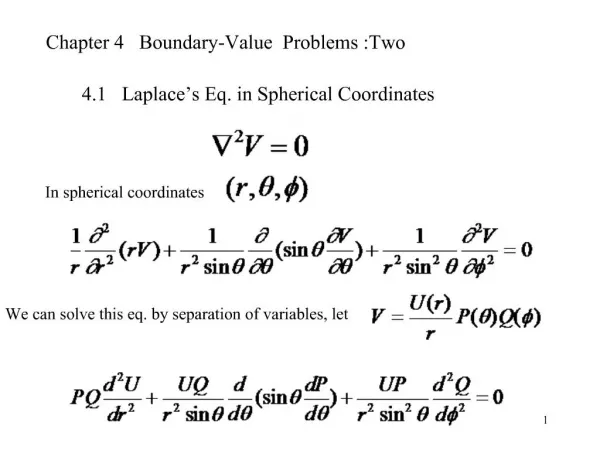
14.3 Problems in Spherical Coordinates: Legendre Polynomials • Laplacian in Spherical Coordinates See Fig 14.15. We knew that (1)and (2)We shall consider only a few of the simpler problems that are independent of the azimuthal angle .
Example 1 • Find the steady-state temperature u(r, ) shown in Fig 14.16.
Example 1 (2) SolutionThe problem is defined as
Example 1 (3) and so (2) (3)After letting x = cos, 0 , (3) becomes (4) This is a form of Legendre’s equation. Now the only solutions of (4) that are continuous and have continuous derivatives on [-1, 1] are the Legendre polynomials Pn(x) corresponding to 2 = n(n+1), n = 0, 1, 2, ….
Example 1 (4) Thus we take the solutions of (3) to be = Pn(cos )When = n(n + 1), the solution of (2) is R = c1 rn + c2 r –(n+1)Since we again expect u to be bounded at r = 0, we define c2 = 0. Hence,
Example 1 (5) Therefore Ancnare the coefficients of the Fourier-Legendre series (23) of Sec 12.5: