Download
1 / 62
650 likes | 2.59k Views
Explore the general features of normal distribution, including standard normal distribution, probability density functions, and practical applications in healthcare. Learn how to interpret data using the normal distribution curve.

E N D
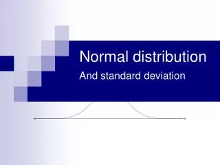
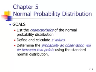
Introduction to continuous probability distributions • Normal distribution and it’s general features • Standard normal distribution • The applications of normal distributions
Section 1-- Introduction to continuous probability distributions
TABLE 2.1 The frequency distribution of weight from 1402 pregnant women
Probability density weight
ffrequency i interval width in frequency distribution table nsample size
When the class intervals become more and more finer, the peak line of histogram will turn into a smooth curve . This is normal distribution. The area under normal curve is 1, because the cumulative percentage is 1.
The characteristics of this family of curves were developed by Abraham de Moivre and karl Friedrich Gauss, so also called Gaussian distribution.
Other examples of normal distribution. • RBC • WBC • Hb • Blood pressure • Height • Weight
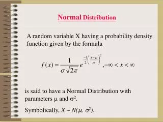
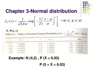
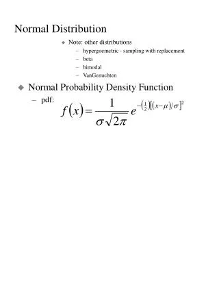
The probability density function for a normal random variable Population mean variance The probability density, or the height of vertical axis Circle rate (3.14258)
If X has a normal distribution with mean μ and standard deviation σ Then we denote this X~N( μ,σ2)
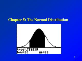
The probability distribution function for a normal random variable The area between -∝ to X1
f(x) x a b
General features of Normal Distribution • 1 The distribution is centered at mean • 2 The distribution is symmetric. • 3 The distribution has two parameters. One is μ( location parameter), the other is σ (variability parameter)
FIG 3 the shift of the graph of the normal density function for various values of μ ,the location parameter
σ =0.5 σ =1 σ =2 FIG 4 the effect on the graph of normal density function of various values of σ ,the “spread” of the distribution linkage
4 The distribution regularity of area under the normal curve Fig 5 the normal curve and it’s area distribution
Normal distribution Standard normal distribution s =1 Z m x
The area under normal curve area (probability) : -the shaded area from negative infinitive to negative Z
General features of Standard Normal Distribution • 1 The distribution is centered at 0 • 2 The distribution is symmetric.
3 The distribution regularity of area under the standard normal curve. Fig 6 the standard normal curve and it’s area distribution
The second decimal place of Z value Combination the number on the column with the corresponding Z value on the row, then Look up cross point
Example 4.1 Suppose that the scores on an aptitude test are normally distributed with a mean of 100 and standard deviation of 10. What is the probability that a randomly selected score is below 90?
Steps Calculate Z Look up Z critical value table and get probability
Solution Transform X into a standard normal variable. μ =100 and σ=10, Thus a score of 90 can be represented as 1 standard deviation below the mean P(X<90)=P(Z<-1.0)
The probability that Z is smaller than -1 is 0.1587, so the probability of a score less than 90 is 15.87%
Example 4.2 What is the probability of a score between 90 and 115?
Solution Transform X into a standard normal variable. μ =100 and σ=10,
We wish to find the shaded area from Z=-1.0 to Z=1.5 15.87% 6.68% 77.45% -1.0 0 1.5 100% - 6.68% - 15.87%= 77.45%
Exercise 1 Suppose that diastolic blood pressure X in hypertensive women centers about 100mmHg and has a standard deviation of 16mmHg and is normally distributed. Find P(X<90) and P(X>124).
Solution Transform X into a standard normal variable. μ =100 and σ=16,
We wish to find the area when Z<-0.625 or Z>1.5 26.43% 6.68% -0.625 0 1.5
1 Estimate reference range 2 Estimate distribution of frequency
1 Estimate reference range (95%) Reference range usually describes the variations of a measurement or value in healthy individuals. It is a basis for a physician or other health professional to interpret a set of results for a particular patient.
Definition of reference range ----The prediction interval between which 95% of values of a reference group fall into, in such a way that 5% of the time a sample value will be beyond this range.
Methods One-sided normal distribution two-sided One-sided <P95Or >P5 Percentile method two-sided P2.5~P97.5
Two-sided values 2.5% of the time a sample value will be less than the lower limit of this interval, and 2.5% of the time it will be larger than the upper limit of this interval Examples: SBP, DBP, Weight……
One-sided values • In many cases, only one side of the range is usually of interest, such as with markers of pathology including cancer antigen, where it is generally without any clinical significance to have a value below what is usual in the population. Therefore, such targets are often given with only one limit of the reference range given, and, strictly, such values are rather cut-off values or threshold values.
Example 4.3 Suppose the concentration of hemoglobin in 120 health women is normally distributed with a mean of 117.4g/L and standard deviation 10.2g/L. What is the 95% reference range of hemoglobin?
Because it is abnormal whether hemoglobin is too higher or too lower. We should use two-sided range. SOLUTION So 95% reference range of hemoglobin is from 97.41 to 137.39g/L