Download
1 / 119
1.44k likes | 2k Views
The Stefan Problem and the Exact Solution for the Two Phase Stefan Problem. DT Project. First Things First. We desire to formulate Two-Phase Stefan Model of Melting and Freezing Non linear model “Moving Boundary Problem” Contains an unknown which is the region to be solved….

E N D
The Stefan Problemand the Exact Solution for the Two Phase Stefan Problem DT Project
First Things First • We desire to formulate Two-Phase Stefan Model of Melting and Freezing • Non linear model • “Moving Boundary Problem” • Contains an unknown which is the region to be solved…..
Why Stefan Problem??? • The formulation of the Stefan Problem is a foundation on which more complex models can be built.
First (cont’d) • Note: • The phase changing process is governed by the conservation of energy. • The unknowns are the temperature field and the location of the Interface. • Involves a phase change material(PCM) with constant density( ), latent heat( ), melt temperature( ), Specific heats( ), and Thermal conductivities( ).
Physical Assumptions • Conduction only • Constant latent heat (L) • Fixed melting temperature( ) which is according to the phase change material (PCM) • Interface thickness is 0 and it is a sharp front; it separates the phases
Assumptions (cont’d) • Thermophysical properties are different for each phase • Conductivities ( ) • Specific heats ( ) • Density remains constant
Other Assumptions • Nucleation and supercooling are assumed to be not present • Surface tension and curvature is insignificant
Only Conduction • Conduction of Heat • Temperature • Heat(enthalphy) • Heat Flux • Characterizes phases
Heat Equation -Heat conduction equation (one space dimension): -well-posed -Heat equation: where
The Two-Phase Stefan Problem • A slab, , initially solid at temperature , is melted by imposing a hot temperature at the face and keeping the back face, insulated (all parameters constant).
Let’s Find a Solution • The solution of the Stefan Problem is T(x,t) and X(t)!!!!
Mathematical Model • PDE for • Interface(t>0) • Initial Condition • Boundary Condition
Be Exact! • In order to explicitly solve the Two-Phase Problem we need to assume the slab is semi-infinite. • Physical Problem: • We want to melt a semi-infinite slab, , initially solid at a temperature , by imposing temperature , on the face . • The “alphas” are different for each phase. All parameters constant.
Mathematical Model • Heat Equations for • Interface(t>0) • Stefan condtion: • Initial Condition • Boundary Condition
Two-Phase Neumann Solution • We derive the Neumann Solution • We use the similarity variable, ,and seek the solution for both for the liquid and for the solid. • Seek a solution for X(t) in the form:
Temperature • Temperature in the liquid region at t>0: • Temperature in the solid region at t>0:
Neumann similarity solution of the 2-phase Stefan Problem for the interface
Transcendental Equation • There is a different Transcendental Equations that incorporates the TWO Stefan numbers (one for each phase). • Trans. Equation: • Stefan Numbers and parameter “v”:
Newton!!! • Newton's method is an algorithm that finds the root of a given function. -Where F(x) = 0. • The fastest way to approximate a root.
What now??? • We can use the Newton algorithm to solve the transcendental equation for the Stefan problem • We do this in order to find a unique root lambda and therefore a unique similarity solution for each
Newton Algorithm • Guess x0 • Take a Newton Step where 3. Terminate if -(Want TOL to be very small so convergence should be noticed) -Stuck. Better guess
Approximate the Root for Newton • For the 2-phase problem there is a good approximation which can be x0 in the Newton program. Approximation of Lambda:
Glauber’s Salt Input Values -Tm = 32; -CpL = 3.31; -CpS = 1.76; -kL = .59e-3; -kS = 2.16e-3; -rho = 1460; -Lat = 251.21; -Tinit = 25; -Tbdy = 90;
Water Input Values - Tm = 0; - CpL = 4.1868; - CpS = .5; - kL = .5664e-3; - kS = 2.16e-3; - rho = 1; - Lat = 333.4;
Glauber’s salt Example maximum number of iterations to be performed,20 tolerance for the residual,1.0e-7 Iterations is 1 xn = 5.170729e-001 fx = -2.740474e-001 Iterations is 2 xn = 5.207715e-001 fx = 1.747621e-002 Iterations is 3 xn = 5.207862e-001 fx = 6.881053e-005 Done. Root is x=5.207862e-001, with Fx=1.068988e-009, Iterations is n=4 LAMBDA= • 5.207861719133929e-001
Plot Lambda vs Stefan For small Stefan numbers from 0:5 and M=51
Portion of Exact Solution Code • function lambda = neumann2p(CpL, CpS, kL, kS, rho, Tm, Lat, Tbdy,Tinit) • format long e • %----------------------Input values--------------------------------------- • CpL = input('Enter specific heat: '); • CpS = input('Enter specific heat of solid: '); • kL = input('Enter thermal conductivity of liquid: '); • kS = input('Enter themal conductivity of solid: '); • rho = input('Enter density which is constant: '); • Tm = input('Enter the melting temperature of substance: '); • Lat = input('Enter Latent heat: '); • TL = input('Enter temperature at x=0: '); • dat2p; • %--------------------------Constants to derive----------------------------- • alphaL = kL/(rho*CpL); • alphaS = kS/ (rho *CpS); • dT = Tbdy - Tm; • dTa = Tm - Tinit; • v = sqrt(alphaL./alphaS); StS = (CpS*dTa)/ Lat; • StL = (CpL*dT)/Lat; • %----------------------------Newton----------------------------------- • x0 = 0.5 * (-StS/ (v*sqrt(pi)) + sqrt(2*StL + (StS/(v*sqrt(pi)))^2)); • lambda = transnewton2p(x0,20,1.0e-7,StS,StL,v); • function Xt = XofT(lambda,alphaL,t) • Xt = 2*lambda*sqrt(alphaL*t); • function TofXTL = TofXTL(lambda,alphaL,Tbdy,dT,x,t) • TofXTL = Tbdy-dT*(erf(x./(2*sqrt(alphaL*t)))./erf(lambda)); • function TofXTS = TofXTS(lambda,alphaS,Tinit,dTa,x,t,v) • TofXTS = Tinit +dTa*(erfc(x./(2*sqrt(alphaS*t)))./erfc(lambda*v))
Exact Histories for Salt -5,10,15 from top to bottom
Exact Profiles for Salt -notice sharp turn at the melt temperature
Formulation/ Discretization of Stefan 2-Phase Problem • Discretize Control Mesh • Discretize Heat Balance • Discretize Fluxes • Discretize Boundary Conditions
Partition Control Volumes: Subdivide the regions into M intervals, or control volumes: with each Subregion associate a node . Volume of :
Discretize Heat Balance Integrating heat balance eq’n over control volume and over time interval
Continue… Dividing out the A and integrating the derivatives yields: Assuming E is uniform and is small:
Discretized Enthalpy From Last Slide: Or
Discretize Fluxes Fourier’s Law: Approximate q discretely:
Discretize Boundary Conditions • Imposing Temperature from left: • Impose exact temperature at back face. • The left boundary flux at x=0: • The right boundary flux at x=l:
Liquid Fraction & “Mushy” • is Solid • is liquid • is “mushy” Liquid Fraction:
Energy & Temperature Relation Solve for T:
Explicit Time Scheme Initial Temperature Known: • Initial Enthalpy Set Resistance and Fluxes from Initial Temperature and Enthalpy Update Enthalpies at Update Temperature Update Liquid Fraction
Update Temperature at Next Time Step: