Download
1 / 42
420 likes | 502 Views
Statistical Process Control. Take periodic samples from a process Plot the sample points on a control chart Determine if the process is within limits Correct the process before defects occur. Common Causes. Assignable Causes. Average. Grams. (a) Mean. Assignable Causes. Average. Grams.

E N D
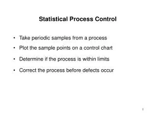
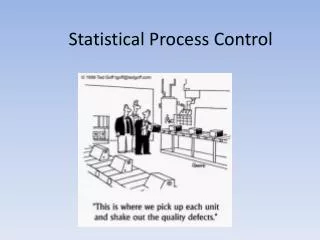
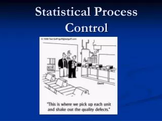
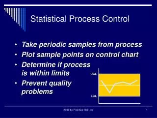
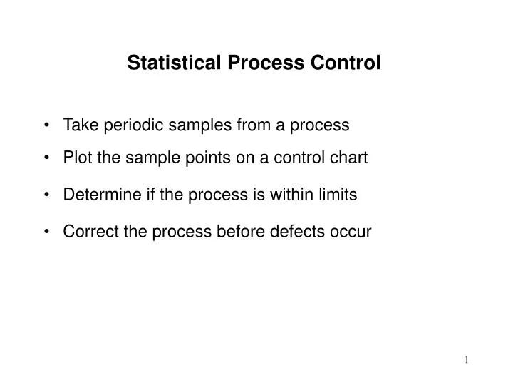
Statistical Process Control • Take periodic samples from a process • Plot the sample points on a control chart • Determine if the process is within limits • Correct the process before defects occur
Assignable Causes Average Grams (a) Mean
Assignable Causes Average Grams (b) Spread
Assignable Causes Average Grams (c) Shape
Control Chart Examples UCL Nominal Variations LCL Sample number
Control Charts Assignable causes likely UCL Nominal LCL 1 2 3 Samples
Mean -3 -2 -1 +1 +2 +3 68.26% 95.44% 99.74% The Normal Distribution = Standard deviation
Control Limits and Errors Type I error: Probability of searching for a cause when none exists UCL Process average LCL (a) Three-sigma limits
Control Limits and Errors Type I error: Probability of searching for a cause when none exists UCL Process average LCL (b) Two-sigma limits
Control Limits and Errors Type II error: Probability of concluding that nothing has changed UCL Shift in process average Process average LCL (a) Three-sigma limits
Control Limits and Errors Type II error: Probability of concluding that nothing has changed UCL Shift in process average Process average LCL (b) Two-sigma limits
Constructing a Control Chart • Decide what to measure or count • Collect the sample data • Plot the samples on a control chart • Calculate and plot the control limits on the control chart • Determine if the data is in-control • If non-random variation is present, discard the data (fix the problem) and recalculate the control limits
Types of Data • Attribute data • Product characteristic evaluated with a discrete choice • Good/bad, yes/no • Variable data • Product characteristic that can be measured • Length, size, weight, height, time, velocity
Control Charts For Attributes • p Charts • Calculate percent defectives in a sample; • an item is either good or bad • c Charts • Count number of defects in an item
p - Charts Based on the binomial distribution
UCL = p + 3 p(1-p) /n = 0.10 + 3 0.10 (1-0.10) /100 = 0.190 p-Chart Calculations Proportion SampleDefect Defective 1 6 .06 2 0 .00 3 4 .04 . . . . . . 20 18 .18 200 • LCL= p - 3 p(1-p) /n • = 0.10 + 3 0.10 (1-0.10) /100 • = 0.010 100 jeans in each sample total defectives total sample observations 200 20 (100) p = = = 0.10
Example p - Chart 0.2 0.18 0.16 0.14 0.12 0.1 Proportion defective 0.08 0.06 0.04 0.02 0 Sample number 0 2 4 6 8 10 12 14 16 18 20 . .
c - Charts Based on the Poisson distribution
c - Chart Calculations Count # of defects per roll in 15 rolls of denim fabric. SampleDefects 1 12 2 8 3 16 . . . . 15 15 190
Example c - Chart 24 21 18 15 . 12 Number of defects 9 6 3 0 0 2 4 6 8 10 12 14 Sample number
Control Charts For Variables • Mean chart (X-Bar Chart) • Measures central tendency of a sample • Range chart (R-Chart) • Measures amount of dispersion in a sample • Each chart measures the process differently. Both the process average and process variability must be in control for the process to be in control.
Example: Control Charts for Variable Data Slip Ring Diameter (cm) Sample 1 2 3 4 5 X R 1 5.02 5.01 4.94 4.99 4.96 4.98 0.08 2 5.01 5.03 5.07 4.95 4.96 5.00 0.12 3 4.99 5.00 4.93 4.92 4.99 4.97 0.08 4 5.03 4.91 5.01 4.98 4.89 4.96 0.14 5 4.95 4.92 5.03 5.05 5.01 4.99 0.13 6 4.97 5.06 5.06 4.96 5.03 5.01 0.10 7 5.05 5.01 5.10 4.96 4.99 5.02 0.14 8 5.09 5.10 5.00 4.99 5.08 5.05 0.11 9 5.14 5.10 4.99 5.08 5.09 5.08 0.15 10 5.01 4.98 5.08 5.07 4.99 5.03 0.10 50.09 1.15
3s Control Chart Factors Sample size X-chart R-chart nA2D3D4 2 1.88 0 3.27 3 1.02 0 2.57 4 0.73 0 2.28 5 0.58 0 2.11 6 0.48 0 2.00 7 0.42 0.08 1.92 8 0.37 0.14 1.86
Process Capability • Range of natural variability in process • Measured with control charts • Process cannot meet specifications if natural variability exceeds tolerances • 3-sigma quality • specifications equal the process control limits. • 6-sigma quality • specifications twice as large as control limits
Process Capability Natural control limits Natural control limits Design specs PROCESS PROCESS Process can meet specifications Process cannot meet specifications Natural control limits Design specs PROCESS Process capability exceeds specifications
Acceptance Sampling Outline • Sampling • Some sampling plans • A single sampling plan • Some definitions • Operating characteristic curve • Developing a single sampling plan
Necessity of Sampling • In most cases 100% inspection is too costly. • In some cases 100% inspection may be impossible. • If only the defective items are returned, repair or replacement may be cheaper than improving quality. But, if the entire lot is returned on the basis of sample quality, then the producer has a much greater motivation to improve quality.
Some Sampling Plans • Single sampling plans: • Most popular and easiest to use • Two numbers n and c • If there are more than c defectives in a sample of size n the lot is rejected; otherwise it is accepted • Double sampling plans: • A sample of size n1 is selected. • If the number of defectives is less than or equal to c1 than the lot is accepted. • Else, another sample of size n2 is drawn. • If the cumulative number of defectives in both samples is more than c2 the lot is rejected; otherwise it is accepted.
Some Sampling Plans • Sequential sampling • An extension of the double sampling plan • Items are sampled one at a time and the cumulative number of defectives is recorded at each stage of the process. • Based on the value of the cumulative number of defectives there are three possible decisions at each stage: • Reject the lot • Accept the lot • Continue sampling
A Single Sampling Plan Consider a single sampling plan with n = 10 and c = 2 • Compute the probability that a lot will be accepted with a proportion of defectives, p = 0.10 • If a producer wants a lot with p = 0.10 to be accepted, the sampling plan has a risk of _______________
A Single Sampling Plan • Compute the probability that a lot will be accepted with a proportion of defectives, p = 0.30 • If a consumer wants to reject a lot with p = 0.30, the sampling plan has a risk of _____________
Some Definitions • Acceptable quality level (AQL) Acceptable fraction defective in a lot • Lot tolerance percent defective (LTPD) Maximum fraction defective accepted in a lot • Producer’s risk, Type I error = P(reject a good lot) • Consumer’s risk, Type II error = P(accept a bad lot)
{ 0.80 0.60 0.40 0.20 { 0.20 0.18 0.02 0.04 0.06 0.08 0.10 0.12 0.14 0.16 Operating Characteristic Curve 1.00 1-a = 0.05 OC curve for n and c Probability of acceptance, Pa b = 0.10 Percent defective AQL LTPD
Example • Develop a sampling plan with AQL = 0.1 LTPD = 0.3 = 0.05 = 0.10
AOQ Curve 0.015 AOQL 0.010 Average Outgoing Quality 0.005 0.10 0.09 0.01 0.02 0.03 0.04 0.05 0.06 0.07 0.08 AQL LTPD (Incoming) Percent Defective
Reading and Exercises • Reading • Chapter 8 pp. 323-36 (self-study) • Technical Note 8 pp. 346-60 • Exercises: • Technical Note Problems 3,12,13