Download
1 / 16
160 likes | 349 Views
Improved Shortest Path Algorithms for Nearly Acyclic Directed Graphs. L. Tian and T. Takaoka University of Canterbury New Zealand 2007. e 1. e 1. e 2. e 2. SC 1. SC 1. SC 2. SC 1. Introduction. What is nearly acyclic directed graphs?

E N D
Improved Shortest Path Algorithms for Nearly Acyclic Directed Graphs L. Tian and T. Takaoka University of Canterbury New Zealand 2007
e1 e1 e2 e2 SC1 SC1 SC2 SC1 Introduction • What is nearly acyclic directed graphs? (1) Takaoka (1998) explained this using a strongly connected component (sc-component) approach, cyc(G). In this example, cyc(G) = 3
Solve the SSSP problem using sc-component decomposition • Compute sc-components Vr,Vr-1, …,V1; • forv∈Vdod[v] ←∞; • d[s]←0; • fori ← r to 1 do{ • Solve the GSS for Gi; • forVj such that (Vi, Vj)∈Edo • forv∈Vi and w∈Vj such that (v, w)∈Edo • d[w] ← min{d[w], d[v] + cost(v,w)}; • } The time complexity of this algorithm is O(m + nlogk), where m is the number of edges in a graph and n is the number of vertices. K is the maximum size of sc components
e1 e2 e3 AC1 AC2 Introduction (continue) (2) Saunders and Takaoka (2005) used a 1-dominator approach to explain that. The SSSP algorithm based on the approach is O(m+rlogr) where r is the number of triggers. e1 e2 e3 AC1 AC2
Restricted Depth First Search for 1-dominator decomposition • functionAcyclicSetA(u){ • VertexSet A, L; • procedurerdfs(v){ • A←A + {v}; • for each w ∈ OUT(A) do{ • ifw LthenL ← L + {w}; // w is visited • inCount[w] ← inCount[w] – 1; • ifinCount[w] = 0 thenrdfs(w); // w is unlocked • } • } • A ← ; L ← {u}; • inCount[u] ← inCount[u] + 1; // prevents re-traversal of u • rdfs(u); • VertexSet B ← L–A; // boundary vertices • for each w ∈ LdoinCount[w] ← |IN(w)|; • return (A,D); • }
Computing the 1-Dominator Set • for all v ∈ VdoinCount[v] ← |IN(v)|; • for all v ∈ VdovertexType[v] ←unknown; • a queue Q← {s}; • whileQ ≠ do{ • Remove the next vertex u from Q; • ifvertexType[u] = unknownthen { • (A, B) ←AcyclicSetA(u); • for each v ∈ Ado Let AC[v] refer to A; • for each v ∈ AdovertexType[v] ←nontrigger; • vertexType[u] ←trigger; • for each v ∈ Bdo • ifvertexType[v] = unknownandvQthen Add v to Q; • } • }
SSSP Algorithm using Acyclic Decomposition • proceduredecreaseKey(u){ • for each v ∈ AC[u] in topological order do • for each w ∈ OUT[v] andw Sdo • d[w] ← min{d[w], d[v] + cost(v,w)}; • } • for all v ∈ Vdod[v] ←∞; • solution set S←; • insert all triggers into frontier set F; • d[s] ← 0; // s is the source vertex • ifs is not a trigger thendecreaseKey(s); • whileF is not empty do{ • find u from F with minimum key and delete u from F; • S ← {u}; • decreaseKey(u); • }
Higher-Order Approach • This approach extends the technique of sc-component decomposition, denoted by cych(G). cyc1(G) cyc2(G) In the second order decomposition, it eats the black node and then decomposes the subgraph.
Higher-Order SSSP Algorithm • procedureDynamic(G, SV){ • Compute hth order sc-components Vhr, Vhr-1, …,Vh1; • fori ← r to 1 do{ • forVhj such that (Vhi, Vhj)∈Ehdo • forv∈Vhi and w∈Vhj such that (v, w)∈Edo • d[w] ← min{d[w], d[v] + cost(v,w)}; • vmin ← w that gives min{d[w] | w ∈Vhi-1 }; • SV ← {vmin }; • if (|Ghi-1|>c1) and (h+1< c2) • then { h ← h+1; Dynamic(Ghi-1; SV); } • else solve the GSS for Ghi-1; • } • } • for all v ∈ Vdod[v] ← ∞; • d[s] ← 0; // s is the source vertex • Dynamic(G, {s});
AC2 AC4 AC1 AC5 AC3 SC1 SC2 Hierarchical Approach • This approach is based on modifications of the sc-component and 1-dominator approaches.
Hierarchical Decomposition Algorithm 1. functionHierarchySets(v0 ) { 2. procedurehdfs(v) { 3. (A, B) ← AcyclicSet(v); 4. Let AC[v] refer to A; 5. vertexType[v] ← trigger ; 6. for all u ∈ A do vertexType[u] ← non-trigger; 7. for all u ∈ Bdo 8. ifvisitNum[u] = 0 do{ 9. c ← c + 1 ; visitNum[u] ← c ; lowlink[u] ← c; 10. T ← T + {u} ; 11. hdfs(u) ; // search from unvisited v ∈ B 12. if u ∈ T thenlowlink[v] ← min(lowlink[u],lowlink[v] ); 13. elselowlink[v] ← min(lowlink[v], vsistNum[u] ); //update lowlink[v] from connected triggers 14. } 15. iflowlink[v] = visitNum[v] andv∈ T do { 16. VertexSet C ← pop up vertices from T until v; 17. p ← p + 1; // count sc-components 18. Let SC[p] refer to C; 19. } 20. } 21. VertexSet AC ← , SC ← , T ← ; 22. for all v ∈ Vdo { 23. inCount[v] ← |IN(v)|; vertexType[v] ← unknown; 24. visitNum[v] ← 0; lowlink[v] ← ; 25. } 26. p ← 0; c ← 0; 27. for all unvisitedv0 ∈ Vdo { 28. c ← c + 1; visitNum[v0] ← c; lowlink[v0 ] ← c; 29. T ← T + v0; 30. hdfs(v0 ); 31. } 32. return(AC, SC, p); 33. }
1-2-dominator sets • Difficulty on 2-dominator sets: • A 1-2-dominator set is a generalization of the 1-dominator set. u1 u1 u2 u3 u2 u3 v1 v1 Vj+1 Vj+1 v2 v2 v3 Vj+2 v3 Vj+2 vj V2j-1 vj V2j-1
Restricted Depth First Search for 1-2-dominator decomposition • functionAcyclicSetA(u){ • VertexSet A, L; • procedurerdfs(v){ • A←A + {v}; • for each w ∈ OUT(A) do{ • ifw LthenL ← L + {w}; // w is visited • inCount[w] ← inCount[w] – 1; • ifinCount[w] = 0 thenrdfs(w); // w is unlocked • } • } • A ← ; L ← {u}; • inCount[u] ← inCount[u] + 1; // prevents re-traversal of u • rdfs(u); • VertexSet B ← L–A; // boundary vertices • for each w ∈ Bdo { 15.1inc(v,w) ← |IN(w)| –inCount[w]; 15.2BS[v] ← (w, inc(v,w)); 15.3 inCount[w] ← |IN(w)|; 15.4 } 16. return (A,B); 17. }
1-2-Dominator Set Algorithm 1. proceduregdfs(u1, u2, v) { 2. for all w ∈ BS[v] do { 3. inCount[w] ← inCount[w] - inc(v, w) ; 4. ifinCount[w] = 0 do { // w is unlocked 5. T1 ← T1 - {w} ; // 1-dominator set T1 6. AC[u1] ← AC[u1] + {w}; 7. AC[u2] ← AC[u2] + {w}; 8. gdfs(u1, u2 , w); 9. } 10. } 11. } /***** main program *****/ 12. Compute 1-dominator set T1 ; 13. foru1 ∈ T1do{ 14. inCount[u1] ← inCount[u1] + 1; 15. for all v ∈ BS[u1] doinCount[v] ← inCount[v] - inc(u1, v); 16 foru2 ∈ T1 - {T1} do { 17. inCount[u1] ← inCount[u2] + 1; 18. gdfs(u1, u2, u2 ); 19. } 20. T1 ← T1 - {u1} ; 21. for all v ∈ BS[u1] doinCount[v] ← |IN(v)|; 22. }
SSSP Algorithm using Acyclic Decomposition • proceduredecreaseKey(u){ • for each v ∈ AC[u] in topological order do • for each w ∈ OUT[v] andw Sdo • d[w] ← min{d[w], d[v] + cost(v,w)}; • } • for all v ∈ Vdod[v] ←∞; • solution set S←; • insert all triggers into frontier set F; • d[s] ← 0; // s is the source vertex • ifs is not a trigger thendecreaseKey(s); • whileF is not empty do{ • find u from F with minimum key and delete u from F; • S ← {u}; • decreaseKey(u); • }
Future research • 1-2-...-k domnator approach: Acyclic structures are dominated by up to k trigger vertices • All Pairs with 1-dominator set O(mn + r2log r) General feedback set approach for all pairs: If we have a feedback vertex set of size r, the best time is O(mn + r3). Conjecture O(mn + r2log r)?