Download

1 / 10
110 likes | 287 Views
Learn about Dijkstra's algorithm for finding shortest paths in weighted graphs, along with its parallel formulations and all pairs shortest paths. Explore the efficiency and speedup of different parallel techniques. Discover the source-parallel technique for improved performance.

E N D
Shortest Path Algorithms Aditya Kumar Sehgal Amlan Bhattacharya
Single Source Shortest Path – Dijkstra’s Algorithm • Weighted graph G = (V, E, w) • Find the shortest paths from a vertex vÎV to all other vertices in V • Edge may represent cost, time, etc. • Dijkstra’s algorithm incrementally finds the shortest path from s to all other vertices • greedy algorithm • similar to Prim’s algorithm for finding minimum spanning tree
Single Source Shortest Path – Dijkstra’s Algorithm procedure DIJKSTRA_SSSP(V, E, w, s) begin VT := {s}; for all vÎ (V – VT) do if (s, v) exists set l[v] := w(s, v); else set l[v] := ¥; whileVT¹Vdo begin find a vertex u such that l[u] := min{l[v] | v Î (V – VT)}; VT := VTÈ {u}; for all vÎ (V – VT) do l[v] := min{l[v], l[u] + w(u, v)}; endwhile end DIJKSTRA_SSSP
Parallel Formulation of Dijkstra’s Algorithm • Similar to parallel formulation of Prim’s algorithm • Let p be number of processors and n be the number of vertices • Divide V into p subsets using 1-D block mapping • each subset has n/p consecutive vertices • work associated with each subset is assigned to a different process • each process stores the part of the array l that corresponds to Vi, where Vi is the subset of vertices assigned to process Pi.
Parallel Formulation of Dijkstra’s Algorithm • Steps • Each process computes li[u] = min{li[v] | vÎ (V – VT) ÇVi} during each iteration of the while loop • Global minimum is obtained over all li[u] by using all-to-one reduction operation and is stored in process P0 • inserted into VT at P0 • P0 broadcasts u to all processes using a one-to-all broadcast • inserted into VT at each Pi • each process updates d[v] for its local vertices • needs to store weight adjacency matrix for columns in Vi • 1-D block mapping of the adjacency matrix at each process
Parallel Formulation of Dijkstra’s Algorithm • Tp = Q(n2/p) + Q(nlogp) • Ts = Q(n2) • Speedup = Q(n2)/Q((n2/p)+(nlogp)) • Efficiency = 1/(1 + Q((plogp)/n))
All Pairs Shortest Paths • Weighted graph G = (V, E, w) • Find the shortest paths between all pairs of vertices vi, vjÎV such that i ¹j • output is an n x n matrix D, where each element Dij is the cost of shortest path between vi and vj
All Pairs Shortest Paths – Dijkstra’s Algorithm • Previously described algorithms can be used • Source Partitioned Formulation • Uses n processes • Each process Pi finds shortest paths from vi to all other vertices using Dijkstra’s sequential SSSP • No communication required • Algorithm can use only n processes • good performance if n = Q (p) • Doesn’t work so well for p > n • Tp = Q(n2) • Speedup = Q(n3)/Q(n2) • Efficiency = Q(1)
All Pairs Shortest Paths – Dijkstra’s Algorithm • Source Parallel Formulation • Major problem with source-partitioned approach is that only n processes can be used • Performance can be improved if parallel version of Dijkstra’s SSSP is used • p processes are divided into n partitions with p/n processes each (p > n) • Each of the n SSSP problems is solved by one of the partitions
All Pairs Shortest Paths – Dijkstra’s Algorithm • Tp = (n3/p) + (nlogp) • Speedup = (n3)/((n3/p) + (nlogp)) • Efficiency = 1/(1 + ((plogp)/n2)) • Source-parallel technique exploits more parallelism that the source-partitioned technique • W = Knplog(p) (pTp – Ts = To) W = KW1/3plog(p) W = K3/2plog(p)3/2 • Better isoefficiency function that source-partitioned function