Download
1 / 30
300 likes | 421 Views
Socio-Economic Scenarios & Climate Change in India Purnamita Dasgupta Institute of Economic Growth, Delhi, India & Johns Hopkins University, USA (Visiting Prof.). Objectives.

E N D
Socio-Economic Scenarios & Climate Change in India Purnamita DasguptaInstitute of Economic Growth, Delhi, India & Johns Hopkins University, USA (Visiting Prof.)
Objectives • Develop alternative socio-economic scenarios that take into consideration a sustainable development objective for India • Focusing on agriculture as a key sector
Methodology • Key markers of socio-economic vulnerability Including Geographical (inter-state variation and coastal location), Demographic (inter-state population distribution) and Coping vulnerability (income differentials and access to education, infrastructure) • Socio-Economic variables impacting the above are then interacted in a dynamic simulation model • Model provides: (a) alternative development pathways through short to medium term projections over (b) varying time scales (c) key parameters which can be influenced to achieve desirable outcomes for decreasing vulnerability, increasing adaptive capacity.
Construct alternative socio-economic scenarios, using simulation modeling Stock and flow diagrams; model construction is done to have enhanced understanding of the inter- relationships between variables Three types of variables in the model: stock, flow and converter; Stocks - show the present state; Flows – variables that change the stocks over time; converters explain the flow
Dynamic model – shows how system is likely to change over time build in the limitations to this growth (climatic factors, other production constraints) Include the capacity to overcome these through adoption of new strategies (technological and policy interventions e.g. increased efficiency of water use)
Conceptual Frame: Dynamic Simulation of Food grain Production Area under Food grain Food Production • Profitability • Technology • Climatic Factors • Irrigation • Other Socio-Economic Factor • Share of Primary Sector • Education • Infrastructure Population Per Capita Production
Gross Domestic Sectoral Product Gross Domestic Product area change due Poverty factor to change in Reduction Share of change in profitability relative Agriculture profitability Sector Food Security, in2 Unemployment Area under Reduction, change in area Foodgrain Acess to Basic foodgrain Services Non irrigated area Population food grain irrigated area foodgrain Proportion of land Per capita irrigated production food <Time> production Yield (irrigated) <Time> Yield <Time> (nonirrigated)
Subsidiary Equations • Area under food grains = f (relative profitability, rainfall, irrigation, educational infrastructure, relative share of primary sector, urbanisation) • Relative profitability = f (relative profitability in past period) • Yield = f (trend, change in technology, change in temperature)
Base year 2004-05; Time series data on major food and non-food crops and related variables for 10 states; 35 years from 1970-71 to 2004-05 Major food crops – paddy, wheat, coarse cereals, pulses. For profitability: All costs in cash and kind including mark up of 10% for managerial functions (opportunity cost); weighted revenue to cost ratio.
Existing secondary data and information collected from government and other agencies both at the national and state level (Census, NAS, Agri. Statistics, Cost of cultivation, UN and RG’s population, district handbooks) Parameter values from existing studies, expert consultation Standard Statistical and econometric techniques for subsidiary equation estimation; qualitative insights Data and Data Analysis
Scenarios A: Reference – no climate change impacts; no major deviations from trend growth rates; current expectations on GDP, population growth B : Optimistic Scenario – higher GDP growth rate, urbanisation; A: Climate Change constrained growth scenario (temperature, precipitation); no intervention B: Growth with adaptation to Climate change (temperature, precipitation)
Assumptions / Constraints • GDP – 9% till 2010, 8% 2020s, 7% 2030s; 6% thereafter • shares in 2030 – agriculture 15%, industry 30%, services 55% • Poverty reduction by 10% (16-17% BPL) by 2012; kept at 5% 2030 onwards • Urbanisation: 40 – 45% in 2030; 50% by 2050 • 100% literacy and 100% access to basic educational and infrastructure services by 2030.
Emerging Scenarios • Time scale from current time period till 2030, 2040, 2050, 2071 • Longer term Scenario – uncertainties
Uncertainty Issues • TFP, technological progress • Limiting – cap values : land availability, irrigation potential, population, relative international prices • Turning points – thresholds : where these lie and extent of certainty of occurrence Quality Assurance • Face Validity through repeated iterations – expected and consistent signs and directions of flows • Historical behaviour tests • Reality checks with extreme values for parameters
Scenarios • A1:Rapid economic growth and rapid introduction of new and more efficient technology, low population growth, substantial reduction in regional differences in per capita income. • A1B: Balanced emphasis on all energy sources.
AIB Data Computation • Data provided at district level, with observation points for each state. The bigger the state, the more the observation points • Available as Monthly and Daily observations • Three time periods: Baseline 1960-1990, Middle 2021-2050, and, Future 2071-2098 • Monthly observations filtered and extracted for Rainfall, Minimum Temperature, Maximum Temperature • Average annual and seasonal rainfall and temperatures calculated across districts • Compiled for each state for the three time periods
Relative Changes in Temperature (2°C or above, Base Year 1960-1990)
State Level Per Capita Foodgrain Production: Reference Scenario
State Level Per Capita Foodgrain Production: Optimistic Scenario
Some Conceptual Concerns • Developmental goals well defined for short term (e.g. MDGs); taken care of in setting the time frames and targets (e.g. literacy, poverty, access to basic amenities) • Adaptation Costs – implies short and medium term cover for derailment of the economy from the desired time path • Socio-economic modeling limitations beyond 2030. Advantage – CC data available, disadvantages – too much uncertainty for socio-economic context (fat tailed pdf with higher probability on extremes, difficulties in cost benefit analysis) Adaptation costs in terms of directions of change, mostly for the long run.