Download
1 / 30
330 likes | 590 Views
Optical flow . Or where do the pixels move?. Alon Gat . Problem Definition. Given: two or more frames of an image sequence Wanted: Displacement field between two consecutive frames optical flow. Visualize Optical Flow.

E N D
Optical flow Or where do the pixels move? Alon Gat
Problem Definition Given: two or more frames of an image sequence Wanted: Displacement field between two consecutive frames optical flow
Visualize Optical Flow Vector Plot: Subsample vector field and use arrows for visualization Color Plot: Visualize direction as color and magnitude as brightness
What is optical flow good for? Extraction of Motion Information • • robot navigation/driver assistance • • surveillance/tracking • • action recognition Processing of Image Sequences • • video compression • • ego motion compensation Related Correspondence Problems • • stereo reconstruction • • structure-from-motion • • medical image registration
How to estimate pixel motion from two images? • Find pixel correspondences • Given a pixel in img1, look for nearby pixels of the same color in img2 • Key assumptions • color constancy: a point in img1 looks “the same” in img2 • For grayscale images, this is brightness constancy • small motion: points do not move very far
Brightness Constancy Assumption Optical Flow: the vector field Displacement: • Assume brightness of patch remains same in both images:
Brightness Constancy Assumption • The LinearizedBrightness Constancy Assumption Idea: If u and v are small and I is sufficiently smooth, one may linearize this constancy assumption via a first-order Taylor expansion around the point Known Unknown
Horn & Schunck Algorithm (MIT 1981) Smoothness Constraint :meaning neighbor pixels in the picture has similar velocities. In other words, nearby pixels moves together
Horn & Schunck Algorithm We seek the set that minimize: Smoothness term Data term brightness constancy • data term - penalizes deviations from constancy assumptions • smoothness term - penalizes dev. from smoothness of the solution • regularization parameter α - determines the degree of smoothness Output – the optical flow!
Smoothing Idea: In order to reduce the influence of noise and outliers, we convolve I0 with a Gaussian of mean μ = 0 and standard deviation Gaussian
Horn & Schunck Algorithm Euler-Lagrange equations According to the calculus of variations, a minimizer of E must fulfill the Euler-Lagrange equations Which are highly non linear system of equations…
Calculus of Variation So we linearize again! Euler-Lagrange equations Or
Horn & Schunck Algorithm flow derivatives here discredited via linear system of equations
Horn & Schunck Algorithm Update Rule:
Problems with the method. • Hard to find boundaries. • Two approximations. Less accurate.
So what are we trying to do? • Instead of approximating the brightness constancy to the 1stTylor expansion, we’ve add one order. • Second and more important, instead of solving E-L equations (which needed to be linearized) we wrote the Functional as n*m equations and minimized it with regular minimization methods (Gradient decent, Quasi Newton, and others)
1. Mathemactica for symbolic calculations. Where P are the Image derivatives, and u, v is the optical flow Mathematica Symbolic Toolbox for MATLAB--Version 2.0 (http://library.wolfram.com/infocenter/MathSource/5344/)
2. Matlab for numeric calculations • Quasi Newton IterationThe problem was that calculation time of inverse of non sparse matrix was long.And then multiplying two non sparse matrix… • Gradient Decent.Non of the above problems but linear convergence rate.And convergence to local min.
3. Leaving Mathematica • In order to get things going faster (moving loooooooong string from matlab to mathematica takes awhile), we found the functional matrix’s constancy and calculate it in matlab. for i=2:imageSizeN-1 for j=2:imageSizeM-1 gradC(i,j)=gradC(i,j)+alpha*(2*(-c(i-1,j)+c(i,j))+2*(-c(i,j-1)+c(i,j))-2*alpha*(-c(i,j)+c(i,j+1)) - 2*alpha*(-c(i,j)+c(i+1,j))+4*exp((-1+c(i,j)^2+s(i,j)^2)^2)*c(i,j)*(-1+c(i,j)^2+s(i,j)^2) +2*(Ix(i,j)*m(i,j)+Ixz(i,j)*m(i,j)+2*Ixx(i,j)*c(i,j)*m(i,j)^2+Ixy(i,j)*m(i,j)^2*s(i,j))*(Iz(i,j)+Izz(i,j)+Ix(i,j)*c(i,j)*m(i,j)+Ixz(i,j)*c(i,j)*m(i,j)+Ixx(i,j)*c(i,j)^2*m(i,j)^2+Iy(i,j)*m(i,j)*s(i,j) +Iyz(i,j)*m(i,j)*s(i,j)+Ixy(i,j)*c(i,j)*m(i,j)^2*s(i,j)+Iyy(i,j)*m(i,j)^2*s(i,j)^2)); gradS(i,j)=gradS(i,j)+4*exp((-1+c(i,j)^2+s(i,j)^2)^2)*s(i,j)*(-1+c(i,j)^2+s(i,j)^2)+2*(Iy(i,j)*m(i,j)+Iyz(i,j)*m(i,j)+Ixy(i,j)*c(i,j)*m(i,j)^2+2*Iyy(i,j)*m(i,j)^2*s(i,j))*(Iz(i,j)+Izz(i,j) +Ix(i,j)*c(i,j)*m(i,j)+Ixz(i,j)*c(i,j)*m(i,j)+Ixx(i,j)*c(i,j)^2*m(i,j)^2+Iy(i,j)*m(i,j)*s(i,j)+Iyz(i,j)*m(i,j)*s(i,j)+Ixy(i,j)*c(i,j)*m(i,j)^2*s(i,j)+Iyy(i,j)*m(i,j)^2*s(i,j)^2) +alpha*(2*(-s(i-1,j)+s(i,j))+2*(-s(i,j-1)+s(i,j))-2*alpha*(-s(i,j)+s(i,j+1))-2*alpha*(-s(i,j)+s(i+1,j))); gradM(i,j)=gradM(i,j)+beta*(2*(-m(i-1,j)+m(i,j))+2*(-m(i,j-1)+m(i,j)))-2*beta*(-m(i,j)+m(i,j+1))-2*beta*(-m(i,j)+m(i+1,j))+2*(Ix(i,j)*c(i,j)+Ixz(i,j)*c(i,j) +2*(Ixx(i,j)*c(i,j)^2*m(i,j)+Iy(i,j)*s(i,j)+Iyz(i,j)*s(i,j)+2*Ixy(i,j)*c(i,j)*m(i,j)*s(i,j)+2*Iyy(i,j)*m(i,j)*s(i,j)^2)*(Iz(i,j)+Izz(i,j)+Ix(i,j)*c(i,j)*m(i,j)+Ixz(i,j)*c(i,j)*m(i,j) +Ixx(i,j)*c(i,j)^2*m(i,j)^2+Iy(i,j)*m(i,j)*s(i,j)+Iyz(i,j)*m(i,j)*s(i,j)+Ixy(i,j)*c(i,j)*m(i,j)^2*s(i,j)+Iyy(i,j)*m(i,j)^2*s(i,j)^2)); end end end
So what is there to optimize? • All methods need couple of unknown parameters which need to be selected by an educated guess. (Condor to the rescue) • All the image derivatives and gradients are calculated in a linear manner.
First results Takes about 45min(highend algorithms take around 20sec…)
Questions? The Ground Truth.