Download
1 / 93
950 likes | 1.22k Views
Digital Image Filters. 26 th Nov ember 2012. Outline. Definitions Linear, shift invariant filters: convolution. Examples of convolutional filters Smoothing Filters ( denoising ) Differentiating Filters (edge detector) Examples of Nonlinear Filtering. Systems.

E N D
Digital Image Filters 26thNovember 2012
Outline • Definitions • Linear, shift invariant filters: convolution. • Examples of convolutional filters • Smoothing Filters (denoising) • Differentiating Filters (edge detector) • Examples of Nonlinear Filtering
Systems • A System H isconsideredasa black box thatprocesses some input signal (f) and gives the output (Hf) • In our case, f isa digital image or a 1-D digitalsignal, but in principlecould be analogic and n-D signalaswellas a scalar
Linearity • A systemissaid to be lineari.i.f. and thishold for all and for aribrarysignals • itis the classicaldefinition of linearity
Signal and System - Property • A systemissaid to be time (or shift) – invarianti.i.f. • Systems that are Linear and TranslationInvariant are represented by a convolutoin. • LTI systems are characterizedentirely by a singlefunction called the system's impulse response. • The impulse response corresponds to the filter associated to the system.
Convolution - LTI System • Let usconsider a signal and a filter • Theirconvolutionis a signal . • For continuous-domain 1D signals and filters i.e., • For discrete signals and filters
Convolution LIT Systems on Images • are discrete 2D signals = Point-wiseproduct sum * • z5 = h9y1+ h8y2 + h7y3 + h6y4 + h5y5 + h5y6 + h3y7 + h2y8 + h1y9
Convolution LIT Systems on Images • are discrete 2D signals = Point-wiseproduct sum * • z5 = h9y1+ h8y2 + h7y3 + h6y4 + h5y5 + h5y6 + h3y7 + h2y8 + h1y9
Convolution LIT Systems on Images • are discrete 2D signals = Point-wiseproduct sum * • z5 = h9y1+ h8y2 + h7y3 + h6y4 + h5y5 + h5y6 + h3y7 + h2y8 + h1y9
Convolution LIT Systems on Images • are discrete 2D signals = Point-wiseproduct sum * • z5 = h9y1+ h8y2 + h7y3 + h6y4 + h5y5 + h5y6 + h3y7 + h2y8 + h1y9
Linear Filters for Digital Images • Linear Filters are particular systems where the output at each pixel (sample) is given by a linear combination of neighboring pixels (samples) Original Signal Filtered Output
Filters or Kernels • The coefficients used in the linear combination are given by the kernel = Image Filter Output Kernel
Linear Filtering -local averaging
Linear Filtering - local averages
Convolution Properties • It is a linear System; it enjoys every LTI properties • Is it Commutative ? but it depends on the patting used. In continuous domain it holds as well as on periodic signals • It is also associative • and dissociative
2D Gaussian Filter Continuous Function Discrete Function
Gaussian Vs Average Gaussian Smoothing Support 7x7 Smoothing by Averaging On 7x7 window
Denoising: The Issue • A Noisy Detail in Camera Raw Data.
Denoising: The Issue • Denoised
Denoising: The Issue • A Noisy Detail in Camera Raw Data.
Denoising: The Issue • Denoised
Image Formation Model • Observation model is • The goal is to obtain , a reliable estimate of , given and the distribution of . • For the sake of simplicity it is often assumed and independent . • The noise standard deviation is assumed as known. Sensed image Pixel index Original (unknown) image noise
Image Formation Model • Observation model is • Thus we can pursue a “regression-approach”,
Image Formation Model • Observation model is • Thuswe can pursue a “regression-approach”, but on images itmaynot be convenient to assume a parametricexpressionof on
Image Formation Model • Observation model is • Thuswe can pursue a “regression-approach”, but on images itmaynot be convenient to assume a parametricexpressionof on
Denoising Approaches • ParametricApproaches • Transform Domain Filtering, they assume the noisy-free signalissomehow sparse in a suitable domain (e.g Fourier, DCT, Wavelet) or w.r.t. some dictionarybaseddecomposition)
Denoising Approaches • ParametricApproaches • Transform Domain Filtering, they assume the noisy-free signalissomehow sparse in a suitable domain (e.g Fourier, DCT, Wavelet) or w.r.t. some dictionarybaseddecomposition) • Non ParametricApproaches • Local Smoothing / Local Approximation • Non Local Methods
Denoising Approaches • ParametricApproaches • Transform Domain Filtering, they assume the noisy-free signalissomehow sparse in a suitable domain (e.g Fourier, DCT, Wavelet) or w.r.t. some dictionarybaseddecomposition) • Non ParametricApproaches • Local Smoothing / Local Approximation • Non Local Methods
Denoising Approaches • ParametricApproaches • Transform Domain Filtering, they assume the noisy-free signalissomehow sparse in a suitable domain (e.g Fourier, DCT, Wavelet) or w.r.t. some dictionarybaseddecomposition) • Non ParametricApproaches • Local Smoothing / Local Approximation • Non Local Methods Estimating from can be statistically treated as regression of on
Fitting and Convolution • One can prove that the leastsquarefit of polynomial of 0-th order (i.econstant) isgiven by where and thus
Denoising Approaches • Non Parametric Approaches: there are no global model for and basically • Local Methods: define, in each image pixel, the “best neighborhood” where a simple parametric model can be enforced to perform regression is described by a (polynomial) model
Ideal neighborhood – an illustrative example • Ideal in the sense that it defines the support of a pointwise Least Square Estimator of the reference point. • Typically, even in simple images, every point has its own different ideal neighborhood. • For practical reasons, the ideal neighborhood is assumedstarshaped Furtherdetailsat LASIP c/o Tampere University of Technology http://www.cs.tut.fi/~lasip/
Neighborhood discretization • A suitablediscretization of thisneighborhoodisobtained by using a set of directional LPA kernels wheredetermines the orientation of the kernelsupport, andwhere controls by the scale of kernel support. Directional kernels Discrete Adaptive Neighborhood Ideal Neighborhood
Neighborhood discretization • A suitablediscretization of thisneighborhoodisobtained by using a set of directional LPA kernels wheredetermines the orientation of the kernelsupport, andwhere controls by the scale of kernel support. • The initial shape optimization problem can be solved by using standard easy-to-implement varying-scale kernel techniques, such as the ICI rule. Directional kernels Discrete Adaptive Neighborhood Ideal Neighborhood
Ideal neighborhood – an illustrative example • Ideal in the sense that it defines the support of pointwise Least Square Estimator of the reference point.
Examples of Adaptively Selected Neighorhoods • Define, , the “ideal” neigborhood • Compute the denoised estimate at , “using”
Examples of adaptively selected neighorhoods • Adaptively selected neighborhoods selected using the LPA-ICI rule