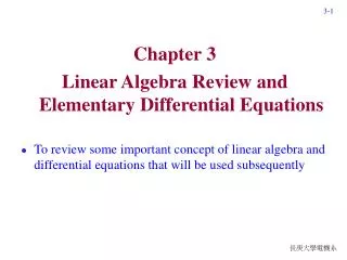
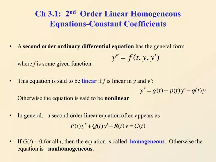
Ch 3.1: 2 nd Order Linear Homogeneous Equations-Constant Coefficients

1. Ch 3.1: 2nd Order Linear Homogeneous Equations-Constant Coefficients • A second order ordinary differential equation has the general form where f is some given function. • This equation is said to be linear if f is linear in y and y': Otherwise the equation is said to be nonlinear. • In general, a second order linear equation often appears as • If G(t) = 0 for all t, then the equation is called homogeneous. Otherwise the equation is nonhomogeneous.

2. Homogeneous Equations, Initial Values • In Sections 3.5 and 3.6, we will see that once a solution to a homogeneous equation is found, then it is possible to solve the corresponding nonhomogeneous equation, or at least express the solution in terms of an integral. • The focus of this chapter is thus on homogeneous equations; and in particular, those with constant coefficients: We will examine the variable coefficient case in Chapter 5. • Initial conditions typically take the form: • Thus, solution passes through (t0, y0), and slope of solution at (t0, y0) is equal to y0'.

3. How do we find a general solution? (Example) Find a solution of the ODE: • (Hint) Consider the first order DE: • Since the two ODEs have constant coefficients, the same kind of functions may be solutions of the ODEs (?) • We will develop rules and principles to get a general solution of a given ODE in Sec 3.2.

4. Example 1: Infinitely Many Solutions (1 of 3) • Consider the second order linear differential equation • Two solutions of this equation are • Other solutions include

5. Example 1: Infinitely Many Solutions (1 of 3) • Consider the second order linear differential equation • Two solutions of this equation are • Other solutions include • Based on these observations, we see that there are infinitely many solutions of the form • It will be shown in Section 3.2 that all solutions of the differential equation above can be expressed in this form (It is called super-position)

6. Example 1: Initial Conditions (2 of 3) • Now consider the following initial value problem for our equation: • We have found a general solution of the form: • Using the initial equations, can we get the coefficients ?

7. Example 1: Initial Conditions (2 of 3) • Now consider the following initial value problem for our equation: • We have found a general solution of the form: • Using the initial equations, • Thus

8. Example 1: Solution Graphs (3 of 3) • Our initial value problem and solution are • Graphs of both y(t) and y’(t) are given below. Observe that both initial conditions are satisfied.

9. Characteristic Equation • To solve the 2nd order equation with constant coefficients, we begin by assuming a solution of the formy = ert. • Substituting this into the differential equation, we obtain • Simplifying, and hence • This last equation is called the characteristic equationof the differential equation. • We then solve for r by factoring or using quadratic formula.

10. General Solution • Using the quadratic formula on the characteristic equation we obtain two solutions, r1 and r2. • There are three possible results: • The roots r1, r2 are real and r1r2. • The roots r1, r2 are real and r1 = r2. • The roots r1, r2 are complex. • In this section, we will assume r1, r2 are real and r1r2. • In this case, the general solution has the form

11. Examples Find solutions of the ODEs (1) (2) (3)

12. Example 2 (case 1: r1r2) • Consider the linear differential equation • Assuming an exponential solution leads to the characteristic equation: • Factoring the characteristic equation yields two solutions: r1 = -2 and r2 = -3 • Therefore, the general solution to this differential equation has the form

13. Initial Conditions • For the initial value problem we use the general solution together with the initial conditions to find c1 and c2. That is, • Since we are assumingr1r2, it follows that a solution of the form y = ert to the above initial value problem will always exist, for any set of initial conditions.

14. Example 3 (IVP) • Consider the initial value problem • From the preceding example, we know the general solution has the form: • With derivative: • Using the initial conditions: • Thus

15. (Ex) Find the solution of the initial value problem

16. Example 4: Initial Value Problem • Consider the initial value problem • Then • Factoring yields two solutions, r1 = 3/2 and r2 = ½ • The general solution has the form • Using initial conditions: • Thus

17. Example 5: Find Maximum Value • For the initial value problem in Example 3, to find the maximum value attained by the solution, we set y’ (t) = 0 and solve for t: