Download
1 / 40
400 likes | 430 Views
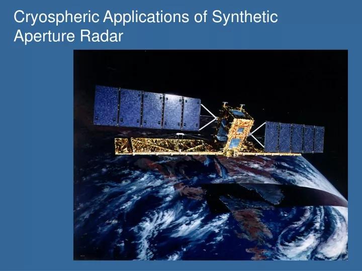
Explore the impact of climate change on Earth's cryospheric regions through SAR technology, enhancing predictive capabilities and understanding ice dynamics for global benefit and decision-making.

E N D
Climate Change and Variability Research for 2015-2020 • If current climate projections are correct, then climate changes of the next ten to twenty years will significantly and noticeably impact human activities. This impact will shift research from climate change detection to research on the predictive capability necessary to protect life and property, promote economic vitality, enable environmental stewardship, and support a broad range of decision-makers. (NRC Decadal Survey, Climate Panel)
Climate Research 2005-2015 • Realization of future climate change forces our decadal vision to extend outside of the current state of the science in several ways: • Climate change research will be increasingly tied to improving predictive capabilities • The drive to create more comprehensive models will grow significantly • The “family” of forecasting products will grow substantially. • The tie between climate research and societal benefit will emphasize regional or higher spatial resolution climate prediction. • The connection between climate and specific impacts on natural and human systems will require a more comprehensive approach to environmental research.
Earth’s Cold Regions and Global Climate • Earth’s cold regions and their icy cover are well documented indicators of climate change • High latitude/elevation processes are important drivers in climate change • Climatologically we are in unfamiliar territory, and the world’s ice cover is responding dramatically. ERS/AMM/MAMM
Science Challenges in Cryospheric Research: • Ice Sheets: Understand the polar ice sheets sufficiently to predict their contribution to global sea level rise. • Sea ice: Understand sea ice sufficiently to predict its response and influence on global climate change and biological processes • Seasonal snow cover: measure how much water is stored as seasonal snow and document its variability • Glaciers: Understand glaciers and ice caps in the context of their hydrologic and biologic systems and their contributions to global processes including sea level rise • Ice and Atmosphere: Understand the interactions between the changing polar atmosphere and the changes in sea ice, glacial ice, snow, and surface melt. • Permafrost: Map extent and variability • As a system: Understand how changes in the cryosphere affect human activity Jacobshavn Fjord, K. Farness, 5/05
Glaciers and Ice Sheets ‘Grand Challenges’ • Understand the polar ice sheets sufficiently to predict their response to global climate change and their contribution global sea level rise • What is the mass balance of the polar ice sheets? • How will the mass balance change in the future?
Reservoirs of Fresh Water Fresh Water Resource Polar Ice Sheets and Glaciers 77% East Antarctica 80% West Antarctica 11% Greenland 8% Glaciers 1% Ice Thickness Average: 2500m Maximum: 4500m National Geographic Magazine
Retreat of Antarctic Ice Sheet and Sea Level Rise Consequences Causes Sea level rise: 6 m Collapse of West Antarctic Ice Sheet Sea level rise: 73 m Melting Entire Antarctic Ice Sheet
Solving the ice sheet problem: Mapping, Surface Properties, Dynamics and Mass Balance Net Accumulation SAR contributes new knowledge about surface structure, ice sheet extent, and surface velocity. Ice In Side Drag Ice out driving stress Surface Topo MAMM InSAR Velocity, Lambert Glacial Basin, 2000 basal drag Bottom Topo
Mass Balance • Ice sheet mass balance is described by the mass continuity equation Altimeters Act/Pass. Microwave InSAR No spaceborne technique available Evaluations of the left and right hand sides of the equation will yield a far more complete result
Ice Dynamics and Prediction Force Balance Equations No Sat. Cover Satellite Altimetry Basal Drag, Inferred at best Terms related to gradients in ice velocity (InSAR) integrated over thickness Understanding dynamics coupled with the continuity equations yields predictions on future changes in mass balance
Radarsat-1 Synthetic Aperture Radar Overview
SAR Imaging Characteristics Range Res ~ pulse width Azimuth = L / 2 ( 25 m resolution with 3 looks) Platform l SEASAT 23 cm HH SIR 23, 5.7, 3.1 cm pol JERS-1 23 cm HH ERS-1/2 5.7 cm VV Radarsat-1 5.7 cm HH ALOS 23 cm pol Radarsat-2 5.7 cm pol TerraSAR-X 3.1 cm pol l 0 e r ’ penetration depth = 2 p e r’’ (several meters even at C-band)
Coherent Properties of SAR • Interferometric SAR measures surface elevation and surface displacement b Velocity q z = r sin( cos-1 f l / 2 p b - q) dz ~ ( df ) r l / 4p b a Topo x z r x = f l / (4p sinb) Fringes are determined by baseline, surface slope, flow speed and flow direction!
Coherent Properties of SAR (cont.) • Phase coherence can be used for change detection < a0 a1* > 0 and 1 denote observations at successive times; mean values computed over many (20 x 4) pixels r = < a0 2 > < a12 > Decorrelation occurs because of: 1) thermal noise; 2) baseline decorrelation; 3) decorrelation of the scattering centers.
Acquisition Planning Instrument Selection Target selection and priority Minimize onboard resources Minimize downlink requirements Conflict resolution
RADARSAT-1 Image Mosaics of Antarctica 2000 1997
Fine Beam Single Look Mini-Mosaics MAMM Mini-Mosaic Orthorectified MAMM Frame AMM-1 Tile
Long Term Change Detection: Coastline Mapping Automatic feature retracking used to create AMM-1 coastline from 25 m data. Portions of MAMM data now also complete Stefansson Bay Utstikkar Glacier 2000 SAR Image AMM-1 MAMM Blocks to date Liu and Jezek
1997 Composite Ice Shelves in the Southeastern Antarctic Peninsula Reclassifying ice tongue and fast ice covered areas as composite ice tongues reduces peninsula ice shelf area by 3500 km2 The composite shelf shown here retreated by 1200 km2 between 1997 and 2000 2000 Jezek, Liu, Thomas, Gogineni, and Krabill
Coastline derived from 1963 DISP Imagery • Accuracy • Image positional accuracy: 2 pixels (200 m) • Relative accuracy of extracted coastline: 1 pixel • Absolute geographical accuracy of extracted coastline: 200 m – 500 m (worst case with light cloud cover) (Kim and Jezek)
Advance and Retreat of Ice Shelves 0.8% decrease in Ice Shelf extent between 1963 and 1997
Continuing the Time Series with MODIS Ross Ice Shelf Margin: 1963 (yellow), 1983/89 (green), 1997 (blue), 2000 (red) coastlines draped over the 2003/04 MOSDIS mosaic.
Short-Term Change Detection: Coherence over 24 days MAMM Coherence Map April, 05 Equivalent range of i and j : Fine beam: 9 x 9 Standard beams: 6 x 24
20 km Dry Valleys Lake Bonney Royal Society Range Bowers Piedmont Gl. Kukri Hills Taylor Valley Ferrar Gl. Lake Fryxell Wilson Piedmont Gl. AMM-1 - Coherence 1997 SAR Mosaic MAMM - Coherence Beam: S2 Look angle: 24.265° Beam: S2 Look angle: 28.152° Coherence variations observable on Ferrar Glacier that are absent in the power image. Lakes are contrast reversed
10 km Dome C MAMM - Coherence 1997 SAR image AMM-1 - Coherence Snow dunes and distinctly different, small scale (10 km) coherence patterns in AMM-1 and MAMM data collected over the interior East Antarctic Ice Sheet. Origin is undetermined..
20 km Decorrelation Stripes 1997 SAR Mosaic MAMM - coherence AMM-1 - coherence Beam: S2 Baseline: 177 m Look angle: 24.265° Beam: S2 Baseline: 149.32 m Look angle: 28.515°
20 km Decorrelation Stripes with the Prevailing Windfield Vector AMM-1 SAR Mosaic Resolution: 100m AMM-1 Coherence Mosaic Resolution: 200m