Download
1 / 33
330 likes | 350 Views
Noise: An Introduction. Adapted from a presentation in: Transmission Systems for Communications , Bell Telephone Laboratories, 1970, Chapter 7. Noise: An Introduction. What is noise? Waveforms with incomplete information Analysis: how? What can we determine?

E N D
Noise: An Introduction Adapted from a presentation in:Transmission Systems for Communications,Bell Telephone Laboratories, 1970, Chapter 7 Noise: An Introduction
Noise: An Introduction • What is noise? • Waveforms with incomplete information • Analysis: how? • What can we determine? • Example: sine waves of unknown phase • Energy Spectral Density • Probability distribution function: P(v) • Probability density function: p(v) • Averages • Common probability density functions • Gaussian • Exponential • Noise in the real-world • Noise Measurement • Energy and Power Spectral densities Noise: An Introduction
BackgroundMaterial • Probability • Discrete • Continuous • The Frequency Domain • Fourier Series • Fourier Transform Noise: An Introduction
Noise • Definition Any undesired signal that interferes with the reproduction of a desired signal • Categories • Deterministic: predictable, often periodic, noise often generated by machines • Random: unpredictable noise, generated by a “stochastic” process in nature or by machines Noise: An Introduction
Random Noise • Unpredictable • “Distribution” of values • Frequency spectrum: distribution of energy (as a function of frequency) • We cannot know the details of the waveform only its “average” behavior Noise: An Introduction
Noise analysis Introduction:a sine wave of unknown phase • Single-frequency interference n(t) = A sin(nt + ) A and n are known, but is not known • We cannot know its value at time “t” Noise: An Introduction
Energy Spectral Density Here the “Energy Spectral Density” is just the magnitude squared of the Fourier transform of n(t) since all of the energy is concentrated at n and each half of the energy is at ± since the Fourier transform is based on the complex exponential not sine and cosine. Noise: An Introduction
Probability Distribution • The “distribution” of the ‘noise” values • Consider the probability that at any time t the voltage is less than or equal to a particular value “v” • The probabilities at some values are easy • P(-A) = 0 • P(A) = 1 • P(0) = ½ • The actual equation is: P(vn) = ½ + (1/)arcsin(vn/A) Shown for A=1 Noise: An Introduction
Probability Distributioncontinued • The actual equation is: P(vn) = ½ + (1/)arcsin(v/A) • Note that the noise spends more time near the extremes and less time near zero. Think of a pendulum: • It stops at the extremes and is moving slowly near them • It move fastest at the bottom and therefore spends less time there. • Another useful function is the derivative of P(vn): the “Probability Density Function”, p(vn) (note the lower case p) Shown for A=1 Noise: An Introduction
Probability Density Function • The area under a portion of this curve is the probability that the voltage lies in that region. • This PDF is zero for|vn| > A Noise: An Introduction
Averages • Time Average of signals • “Ensemble” Average • Assemble a large number of examples of the noise signal. (the set of all examples is the “ensemble”) • At any particular time (t0) average the set of values of vn(t0) to get the “Expected Value” of vn • When the time and ensemble averages give the same value (they usually do), the noise process is said to be “Ergodic” Noise: An Introduction
Averages (2) • Now calculate the ensemble average of our sinusoidal “noise” • Which is obviously zero (odd symmetry, balance point, etc.as it should since this noise the has no DC component.) Noise: An Introduction
Averages (3) • E[vn] is also known as the “First Moment” of p(vn) • We can also calculate other important moments of p(vn). The “Second Central Moment” or “Variance” (2) is:Which for our sinusoidal noise is: Noise: An Introduction
Averages (4) Integrating this requires “Integration by parts 0 Noise: An Introduction
Averages (5) Continuing Which corresponds to the power of our sine wave noise Note: (without the “squared”) is called the “Standard Deviation” of the noise and corresponds to the RMS value of the noise Noise: An Introduction
Common Probability Density Functions:The Gaussian Distribution • Central Limit Theorem The probability density function for a random variable that is the result of adding the effects of many small contributors tends to be Gaussian as the number of contributors gets large. Noise: An Introduction
Common Probability Density Functions:The Exponential Distribution • Occurs naturally in discrete “Poisson Processes” • Time between occurrences • Telephone calls • Packets Noise: An Introduction
Common Noise Signals • Thermal Noise • Shot Noise • 1/f Noise • Impulse Noise Noise: An Introduction
Thermal Noise • From the Brownian motion of electrons in a resistive material. pn(f) = kT is the power spectrumwhere: k = 1.3805 * 10-23 (Boltzmann’s constant) and T is the absolute temperature (°Kelvin) • This is a “white” noise (“flat” spectrum) • From a color analogy • White light has all colors at equal energy • The probability distribution is Gaussian Noise: An Introduction
Thermal Noise (2) • A more accurate model (Quantum Theory) Which corrects for the high frequency roll off(above 4000 GHz at room temperature) • The power in the noise is simply Pn = k*T*BW Watts or Pn = -174 + 10*log10(BW) in dBm (decibels relative to a milliwatt) Note: dB = 10*log10 (P/Pref ) = 20*log10 (V/Vref ) Noise: An Introduction
Shot Noise • From the irregular flow of electrons Irms = 2*q*I*f where: q = 1.6 * 10-19 the charge on an electron • This noise is proportional to the signal level(not temperature) • It is also white (flat spectrum) and Gaussian Noise: An Introduction
1/f Noise • Generated by: • irregularities in semiconductor doping • contact noise • Models many naturally occurring signals • “speech” • Textured silhouettes (Mountains, clouds, rocky walls, forests, etc.) • pn(f) =A / f (0.8 < < 1.5) Noise: An Introduction
Impulse Noise • Random energy spikes, clicks and pops • Common sources • Lightning • Vehicle ignition systems • This is a white noise, but NOT Gaussian • Adding multiple sources - more impulse noise • An exception to the “Central Limit Theorem” Noise: An Introduction
Noise Measurement • The Human Ear • Average Performance • The Cochlea • Hearing Loss • Noise Level • A-Weighted • C-Weighted Noise: An Introduction
Hearing Performance(an average, good, ear) • Frequency response is a function of sound level • 0 dB here is the threshold of hearing • Higher intensities yield flatter response Noise: An Introduction
The Cochlea • A fluid-filled spiral vibration sensor • Spatial filter: • Low frequencies travel the full length • High frequencies only affect the near end • Cillia: hairs put out signals when moved • Hearing damage occurs when these are injured • Those at the near end are easily damaged (high frequency hearing loss) Noise: An Introduction
Noise Intensity Levels:The A- Weighted Filter • Corresponds to the sensitivity of the ear at the threshold of hearing; used to specify OSHA safety levels (dBA) Noise: An Introduction
An A-Weighting Filter • Below is an active filter that will accurately perform A-Weighting for sound measurementsThanks to: Rod Elliottat http://sound.westhost.com/project17.htm Noise: An Introduction
Noise Intensity Levels:The C- Weighted Filter • Corresponds to the sensitivity of the ear at normal listening levels; used to specify noise in telephone systems (dBC) Noise: An Introduction
Energy Spectral Density (ESD) Noise: An Introduction
Energy Spectral Density (ESD)and Linear Systems X(w) Y(w) = X(w) H(w) H(w) Therefore the ESD of the output of a linear system is obtained by multiplying the ESD of the input by |H(w)|2 Noise: An Introduction
Power Spectral Density (PSD) • Functions that exist for all time have an infinite energy so we define power as: Noise: An Introduction
Power Spectral Density (PSD-2) • As before, the function in the integral is a density. This time it’s the PSD • Both the ESD and PSD functions are real and even functions Noise: An Introduction