Download

1 / 42
420 likes | 491 Views
Learn the characteristics of one-factor experiments, when to avoid them, and an example experiment. Calculate errors, effects, and variations to interpret results accurately. Find out how to allocate and assign variation in experiments to improve analysis.

E N D
One-Factor Experiments Andy Wang CIS 5930 Computer Systems Performance Analysis
Characteristics ofOne-Factor Experiments • Useful if there’s only one important categorical factor with more than two interesting alternatives • Methods reduce to 21 factorial designs if only two choices • If single variable isn’t categorical, should use regression instead • Method allows multiple replications
Comparing Truly Comparable Options • Evaluating single workload on multiple machines • Trying different options for single component • Applying single suite of programs to different compilers
When to Avoid It • Incomparable “factors” • E.g., measuring vastly different workloads on single system • Numerical factors • Won’t predict any untested levels • Regression usually better choice • Related entries across level • Use two-factor design instead
An Example One-Factor Experiment • Choosing authentication server for single-sized messages • Four different servers are available • Performance measured by response time • Lower is better
The One-Factor Model • yij = j + eij • yij is ith response with factor set at level j • Each level is a server type • is mean response • j is effect of alternative j • How the mean of each alternative different from • eij is error term
One-Factor Experiments With Replications • Initially, assume r replications at each alternative of factor • Assuming a alternatives, we have a total of ar observations • Model is thus
Sample Datafor Our Example • Four server types, with four replications each (measured in seconds) A B C D 0.96 0.75 1.01 0.93 1.05 1.22 0.89 1.02 0.82 1.13 0.94 1.06 0.94 0.98 1.38 1.21
Computing Effects • Need to figure out and j • We have various yij’s • Errors should add to zero: • Similarly, effects should add to zero:
Calculating • By definition, sum of errors and sum of effects are both zero, • And thus, is equal to grand mean of all responses
Calculating j • j is vector of responses • One for each alternative of the factor • To find vector, find column means • Separate mean for each j • Can calculate directly from observations
Calculating Column Mean • We know that yij is defined to be • So,
Calculating Parameters • Sum of errors for any given row is zero, so • So we can solve for j:
Parametersfor Our Example Server A B C D Col. Mean .9425 1.02 1.055 1.055 Subtract from column means to get parameters Parameters -.076 .002 .037 .037
EstimatingExperimental Errors • Estimated response is • But we measured actual responses • Multiple ones per alternative • So we can estimate amount of error in estimated response • Use methods similar to those used in other types of experiment designs
Sum of Squared Errors • SSE estimates variance of the errors: • We can calculate SSE directly from model and observations • Also can find indirectly from its relationship to other error terms
SSE for Our Example • Calculated directly: SSE = (.96-(1.018-.076))^2 + (1.05 - (1.018-.076))^2 + . . . + (.75-(1.018+.002))^2 + (1.22 - (1.018 + .002))^2 + . . . + (.93 -(1.018+.037))^2 = .3425
Allocating Variation • To allocate variation for model, start by squaring both sides of model equation • Cross-product terms add up to zero
Variation In Sum of Squares Terms • SSY = SS0 + SSA + SSE • Gives another way to calculate SSE
Sum of Squares Termsfor Our Example • SSY = 16.9615 • SS0 = 16.58256 • SSA = .03377 • So SSE must equal 16.9615-16.58256-.03377 • I.e., 0.3425 • Matches our earlier SSE calculation
Assigning Variation • SST is total variation • SST = SSY - SS0 = SSA + SSE • Part of total variation comes from model • Part comes from experimental errors • A good model explains a lot of variation
Assigning Variationin Our Example • SST = SSY - SS0 = 0.376244 • SSA = .03377 • SSE = .3425 • Percentage of variation explained by server choice
Analysis of Variance • Percentage of variation explained can be large or small • Regardless of which, may or may not be statistically significant • To determine significance, use ANOVA procedure • Assumes normally distributed errors
Running ANOVA • Easiest to set up tabular method • Like method used in regression models • Only slight differences • Basically, determine ratio of Mean Squared of A (parameters) to Mean Squared Errors • Then check against F-table value for number of degrees of freedom
ANOVA Table forOne-Factor Experiments Compo- Sum of % of Degrees of Mean F- F- nent Squares Var. Freedom Square Comp Table yar 1 SST=SSY-SS0 100 ar-1 Aa-1 F[1-; a-1,a(r-1)] e SSE=SST-SSA a(r-1)
ANOVA Procedurefor Our Example Compo- Sum of % of Degrees of Mean F- F- nent Squares Variation Freedom Square Comp Table y 16.96 16 16.58 1 .376 100 15 A .034 8.97 3 .011 .394 2.61 e .342 91.0 12 .028
Interpretationof Sample ANOVA • Done at 90% level • F-computed is .394 • Table entry at 90% level with n=3 and m=12 is 2.61 • Thus, servers are not significantly different
One-Factor Experiment Assumptions • Analysis of one-factor experiments makes the usual assumptions: • Effects of factors are additive • Errors are additive • Errors are independent of factor alternatives • Errors are normally distributed • Errors have same variance at all alternatives • How do we tell if these are correct?
Visual Diagnostic Tests • Similar to those done before • Residuals vs. predicted response • Normal quantile-quantile plot • Residuals vs. experiment number
What Does The Plot Tell Us? • Analysis assumed size of errors was unrelated to factor alternatives • Plot tells us something entirely different • Very different spread of residuals for different factors • Thus, one-factor analysis is not appropriate for this data • Compare individual alternatives instead • Use pairwise confidence intervals
Could We Have Figured This Out Sooner? • Yes! • Look at original data • Look at calculated parameters • Model says C & D are identical • Even cursory examination of data suggests otherwise
Looking Back at the Data A B C D 0.96 0.75 1.01 0.93 1.05 1.22 0.89 1.02 0.82 1.13 0.94 1.06 0.94 0.98 1.38 1.21 Parameters -.076 .002 .037 .037
What Does This PlotTell Us? • Overall, errors are normally distributed • If we only did quantile-quantile plot, we’d think everything was fine • The lesson - test ALL assumptions, not just one or two
One-Factor Confidence Intervals • Estimated parameters are random variables • Thus, can compute confidence intervals • Basic method is same as for confidence intervals on 2kr design effects • Find standard deviation of parameters • Use that to calculate confidence intervals • Typo in book, pg 336, example 20.6, in formula for calculating j • Also typo on pg. 335: degrees of freedom is a(r-1), not r(a-1)
Confidence Intervals For Example Parameters • se = .169 • Standard deviation of = .042 • Standard deviation of j = .073 • 95% confidence interval for = (.932, 1.10) • 95% CI for = (-.225, .074) • 95% CI for = (-.148,.151) • 95% CI for = (-.113,.186) • 95% CI for = (-.113,.186)
Unequal Sample Sizes in One-Factor Experiments • Don’t really need identical replications for all alternatives • Only slight extra difficulty • See book example for full details
Changes To HandleUnequal Sample Sizes • Model is the same • Effects are weighted by number of replications for that alternative: • Slightly different formulas for degrees of freedom