Introduction to Survival Analysis: Key Concepts and Methods

1. Introduction to Survival AnalysisOctober 19, 2004 Brian F. Gage, MD, MSc with thanks to Bing Ho, MD, MPH Division of General Medical Sciences

2. Presentation goals • Survival analysis compared w/ other regression techniques • What is survival analysis • When to use survival analysis • Univariate method: Kaplan-Meier curves • Multivariate methods: • Cox-proportional hazards model • Parametric models • Assessment of adequacy of analysis • Examples

3. Regression vs. Survival Analysis

4. Regression vs. Survival Analysis

5. What is survival analysis? • Model time to failure or time to event • Unlike linear regression, survival analysis has a dichotomous (binary) outcome • Unlike logistic regression, survival analysis analyzes the time to an event • Why is that important? • Able to account for censoring • Can compare survival between 2+ groups • Assess relationship between covariates and survival time

6. Importance of censored data • Why is censored data important? • What is the key assumption of censoring?

7. Types of censoring • Subject does not experience event of interest • Incomplete follow-up • Lost to follow-up • Withdraws from study • Dies (if not being studied) • Left or right censored

8. When to use survival analysis • Examples • Time to death or clinical endpoint • Time in remission after treatment of disease • Recidivism rate after addiction treatment • When one believes that 1+ explanatory variable(s) explains the differences in time to an event • Especially when follow-up is incomplete or variable

9. Relationship between survivor function and hazard function • Survivor function, S(t) defines the probability of surviving longer than time t • this is what the Kaplan-Meier curves show. • Hazard function is the derivative of the survivor function over time h(t)=dS(t)/dt • instantaneous risk of event at time t (conditional failure rate) • Survivor and hazard functions can be converted into each other

10. Approach to survival analysis • Like other statistics we have studied we can do any of the following w/ survival analysis: • Descriptive statistics • Univariate statistics • Multivariate statistics

11. Descriptive statistics • Average survival • When can this be calculated? • What test would you use to compare average survival between 2 cohorts? • Average hazard rate • Total # of failures divided by observed survival time (units are therefore 1/t or 1/pt-yrs) • An incidence rate, with a higher values indicating more events per time

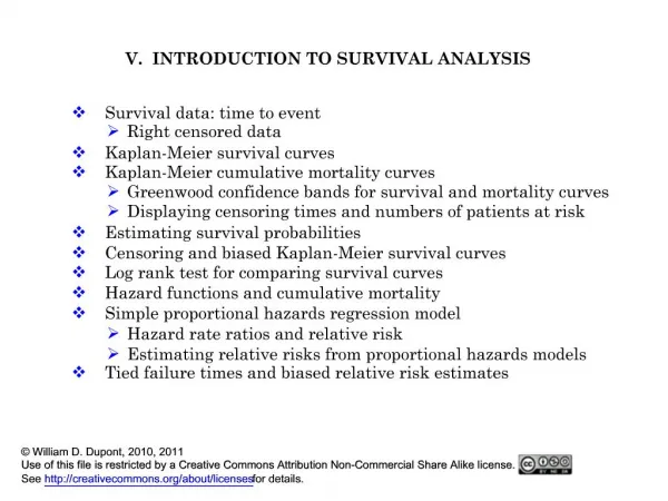
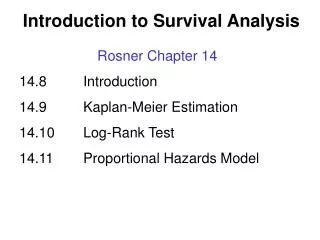
12. Univariate method: Kaplan-Meier survival curves • Also known as product-limit formula • Accounts for censoring • Generates the characteristic “stair step” survival curves • Does not account for confounding or effect modification by other covariates • When is that a problem? • When is that OK?

14. Time to Cardiovascular Adverse Event in VIGOR Trial

16. Comparing Kaplan-Meier curves • Log-rank test can be used to compare survival curves • Less-commonly used test: Wilcoxon, which places greater weights on events near time 0. • Hypothesis test (test of significance) • H0: the curves are statistically the same • H1: the curves are statistically different • Compares observed to expected cell counts • Test statistic which is compared to 2 distribution

17. Comparing multiple Kaplan-Meier curves • Multiple pair-wise comparisons produce cumulative Type I error – multiple comparison problem • Instead, compare all curves at once • analogous to using ANOVA to compare > 2 cohorts • Then use judicious pair-wise testing

18. Limit of Kaplan-Meier curves • What happens when you have several covariates that you believe contribute to survival? • Example • Smoking, hyperlipidemia, diabetes, hypertension, contribute to time to myocardial infarct • Can use stratified K-M curves – for 2 or maybe 3 covariates • Need another approach – multivariate Cox proportional hazards model is most common -- for many covariates • (think multivariate regression or logistic regression rather than a Student’s t-test or the odds ratio from a 2 x 2 table)

19. Multivariate method: Cox proportional hazards • Needed to assess effect of multiple covariates on survival • Cox-proportional hazards is the most commonly used multivariate survival method • Easy to implement in SPSS, Stata, or SAS • Parametric approaches are an alternative, but they require stronger assumptions about h(t).

20. Cox proportional hazard model • Works with hazard model • Conveniently separates baseline hazard function from covariates • Baseline hazard function over time • h(t) = ho(t)exp(B1X+Bo) • Covariates are time independent • B1 is used to calculate the hazard ratio, which is similar to the relative risk • Nonparametric • Quasi-likelihood function

21. Cox proportional hazards model, continued • Can handle both continuous and categorical predictor variables (think: logistic, linear regression) • Without knowing baseline hazard ho(t), can still calculate coefficients for each covariate, and therefore hazard ratio • Assumes multiplicative risk—this is the proportional hazard assumption • Can be compensated in part with interaction terms

22. Limitations of Cox PH model • Does not accommodate variables that change over time • Luckily most variables (e.g. gender, ethnicity, or congenital condition) are constant • If necessary, one can program time-dependent variables • When might you want this? • Baseline hazard function, ho(t), is never specified • You can estimate ho(t) accurately if you need to estimate S(t).

23. Hazard ratio • What is the hazard ratio and how to you calculate it from your parameters, β • How do we estimate the relative risk from the hazard ratio (HR)? • How do you determine significance of the hazard ratios (HRs). • Confidence intervals • Chi square test

24. Assessing model adequacy • Multiplicative assumption • Proportional assumption: covariates are independent with respect to time and their hazards are constant over time • Three general ways to examine model adequacy • Graphically • Mathematically • Computationally: Time-dependent variables (extended model)

25. Model adequacy: graphical approaches • Several graphical approaches • Do the survival curves intersect? • Log-minus-log plots • Observed vs. expected plots

26. Testing model adequacy mathematically with a goodness-of-fit test • Uses a test of significance (hypothesis test) • One-degree of freedom chi-square distribution • p value for each coefficient • Does not discriminate how a coefficient might deviate from the PH assumption

27. Example: Tumor Extent • 3000 patients derived from SEER cancer registry and Medicare billing information • Exploring the relationship between tumor extent and survival • Hypothesis is that more extensive tumor involvement is related to poorer survival

28. Log-Rank 2 = 269.0973 p <.0001

29. Example: Tumor Extent • Tumor extent may not be the only covariate that affects survival • Multiple medical comorbidities may be associated with poorer outcome • Ethnic and gender differences may contribute • Cox proportional hazards model can quantify these relationships

30. Example: Tumor Extent • Test proportional hazards assumption with log-minus-log plot • Perform Cox PH regression • Examine significant coefficients and corresponding hazard ratios

32. Example: Tumor Extent 5 The PHREG Procedure Analysis of Maximum Likelihood Estimates Parameter Standard Hazard 95% Hazard Ratio Variable Variable DF Estimate Error Chi-Square Pr > ChiSq Ratio Confidence Limits Label age2 1 0.15690 0.05079 9.5430 0.0020 1.170 1.059 1.292 70<age<=80 age3 1 0.58385 0.06746 74.9127 <.0001 1.793 1.571 2.046 age>80 race2 1 0.16088 0.07953 4.0921 0.0431 1.175 1.005 1.373 black race3 1 0.05060 0.09590 0.2784 0.5977 1.052 0.872 1.269 other comorb1 1 0.27087 0.05678 22.7549 <.0001 1.311 1.173 1.465 comorb2 1 0.32271 0.06341 25.9046 <.0001 1.381 1.219 1.564 comorb3 1 0.61752 0.06768 83.2558 <.0001 1.854 1.624 2.117 DISTANT 1 0.86213 0.07300 139.4874 <.0001 2.368 2.052 2.732 REGIONAL 1 0.51143 0.05016 103.9513 <.0001 1.668 1.512 1.840 LIPORAL 1 0.28228 0.05575 25.6366 <.0001 1.326 1.189 1.479 PHARYNX 1 0.43196 0.05787 55.7206 <.0001 1.540 1.375 1.725 treat3 1 0.07890 0.06423 1.5090 0.2193 1.082 0.954 1.227 both treat2 1 0.47215 0.06074 60.4215 <.0001 1.603 1.423 1.806 rad treat0 1 1.52773 0.08031 361.8522 <.0001 4.608 3.937 5.393 none

33. Summary • Survival analyses quantifies time to a single, dichotomous event • Handles censored data well • Survival and hazard can be mathematically converted to each other • Kaplan-Meier survival curves can be compared statistically and graphically • Cox proportional hazards models help distinguish individual contributions of covariates on survival, provided certain assumptions are met.