Download
1 / 41
440 likes | 615 Views
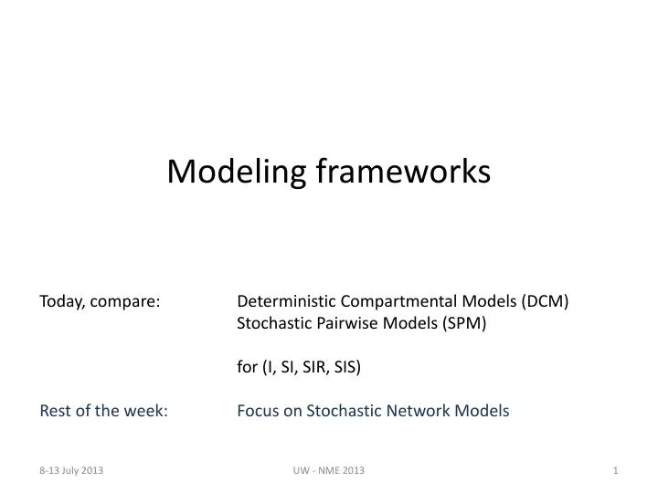
Modeling frameworks. Today, compare: Deterministic Compartmental Models (DCM) Stochastic Pairwise Models (SPM) for (I, SI, SIR, SIS) R est of the week: Focus on Stochastic Network Models. Deterministic Compartmental Modeling. Susceptible. Infected. Recovered.

E N D
Modeling frameworks Today, compare: Deterministic Compartmental Models (DCM) Stochastic Pairwise Models (SPM) for (I, SI, SIR, SIS) Rest of the week: Focus on Stochastic Network Models UW - NME 2013
Deterministic Compartmental Modeling Susceptible Infected Recovered UW - NME 2013
Compartmental Modeling • A form of dynamic modeling in which people are divided up into a limited number of “compartments.” • Compartments may differ from each other on any variable that is of epidemiological relevance (e.g. susceptible vs. infected, male vs. female). • Within each compartment, people are considered to be homogeneous, and considered only in the aggregate. Compartment 1 UW - NME 2013
Compartmental Modeling • People can move between compartments along “flows”. • Flows represent different phenomena depending on the compartments that they connect • Flow can also come in from outside the model, or move out of the model • Most flows are typically a function of the size of compartments Susceptible Infected UW - NME 2013
Compartmental Modeling • May be discrete time or continuous time: we will focus on discrete • The approach is usually deterministic – one will get the exact same results from a model each time one runs it • Measures are always of EXPECTED counts – that is, the average you would expect across many different stochastic runs, if you did them • This means that compartments do not have to represent whole numbers of people. UW - NME 2013
Constant-growth model Infected population t = time i(t) = expected number of infected people at time t k = average growth (in number of people) per time period UW - NME 2013
Constant-growth model difference equation (three different notations for the same concept – keep all in mind when reading the literature!) recurrence equation UW - NME 2013
Example: Constant-growth model i(0) = 0; k = 7 UW - NME 2013
Proportional growth model Infected population t = time i(t) = expected number of infected people at time t r= average growth rate per time period difference equation recurrence equation UW - NME 2013
Example: Proportional-growth model i(1) = 1; r = 0.3 UW - NME 2013
SI model New infections per unit time (incidence) Susceptible Infected t = time s(t) = expected number of susceptible people at time t i(t) = expected number of infected people at time t What is the expected incidence per unit time? UW - NME 2013
SI model t = time s(t) = expected number of susceptible people at time t i(t) = expected number of infected people at time t A new infection requires: a susceptible person to have an act with an infected person and for infection to transmit because of that act Expected incidence at time t UW - NME 2013
SI model t = time s(t) = expected number of susceptible people at time t i(t) = expected number of infected people at time t A new infection requires: a susceptible person to have an act with an infected person and for infection to transmit because of that act Expected incidence at time t UW - NME 2013
SI model t = time s(t) = expected number of susceptible people at time t i(t) = expected number of infected people at time t = act rate per unit time A new infection requires: a susceptible person to have an act with an infected person and for infection to transmit because of that act Expected incidence at time t UW - NME 2013
SI model t = time s(t) = expected number of susceptible people at time t i(t) = expected number of infected people at time t = act rate per unit time A new infection requires: a susceptible person to have an act with an infected person and for infection to transmit because of that act Expected incidence at time t UW - NME 2013
SI model t = time s(t) = expected number of susceptible people at time t i(t) = expected number of infected people at time t = act rate per unit time = “transmissibility” = prob. of transmission given S-I act A new infection requires: a susceptible person to have an act with an infected person and for infection to transmit because of that act Expected incidence at time t UW - NME 2013
SI model t = time s(t) = expected number of susceptible people at time t i(t) = expected number of infected people at time t = act rate per unit time = “transmissibility” = prob. of transmission given S-I act n(t) = total population = s(t) + i(t) A new infection requires: a susceptible person to have an act with an infected person and for infection to transmit because of that act Expected incidence at time t UW - NME 2013
SI model t = time s(t) = expected number of susceptible people at time t i(t) = expected number of infected people at time t = act rate per unit time = “transmissibility” = prob. of transmission given S-I act n(t) = total population = s(t) + i(t) = n A new infection requires: a susceptible person to have an act with an infected person and for infection to transmit because of that act Expected incidence at time t Careful: only because this is a “closed”population UW - NME 2013
SI model Susceptible Infected Expected incidence at time t What does this mean for our system of equations? UW - NME 2013
SI model Susceptible Infected Expected incidence at time t What does this mean for our system of equations? UW - NME 2013
SI model - Recurrence equations Remember: constant-growth model could be expressed as: proportional-growth model could be expressed as: The SI model is very simple, but already too difficult to express as a simple recurrence equation. Solving iteratively by hand (or rather, by computer) is necessary UW - NME 2013
SIR model What if infected people can recover with immunity? Susceptible Infected Recovered And let us assume they all do so at the same rate: t = time s(t) = expected number of susceptible people at time t i(t) = expected number of infected people at time t r(t) = expected number of recovered people at time t = act rate per unit time = prob. of transmission given S-I act r = recovery rate UW - NME 2013
Relationship between duration and recovery rate • Imagine that a disease has a constant recover rate of 0.2. That is, on the first day of infection, you have a 20% probability of recovering. If you don’t recover the first day, you then have a 20% probability of recovering on Day 2. Etc. • Now, imagine 100 people who start out sick on the same day. • How many recover after being infected 1 day? • How many recover after being infected 2 days? • How many recover after being infected 3 days? • What does the distribution of time spent infected look like? • What is this distribution called? • What is the mean (expected) duration spent sick? 100*0.2 = 20 80*0.2 = 16 64*0.2 = 12.8 Right-tailed Geometric 5 days ( = 1/.2) D = 1/ r UW - NME 2013
SIR model Expected number of new infections at time t still equals where nnow equals Expected number of recoveries at time t equals So full set of equations equals: UW - NME 2013
SIR model = 0.6, = 0.3, = 0.1 Initial population sizes s(0)=299; i(0)=1; r(0) = 0 susceptible recovered infected What happens on Day 62? Why? UW - NME 2013
Qualitative analysis pt 1: Epidemic potential Using the SIR model • R0= the number of direct infections occurring as a result of a single infection in a susceptible population – that is, one that has not experienced the disease before • We saw earlier that R0= . So for the basic SIR model, it also equals / • Tells one whether an epidemic is likely to occur or not: • If R0 > 1, then a single infected individual in the population will on average infect more than one person before ceasing to be infected. In a deterministic model, the disease will grow • If R0 < 1, then a single infected individual in the population will on average infect less than one person before ceasing to be infected. In a deterministic model, the disease will fade away • If R0 = 1, we are right on the threshold between an epidemic and not. In a deterministic model, the disease will putter along UW - NME 2013
SIR model = 4, = 0.2, = 0.2 Initial population sizes s(0)=999; i(0)=1; r(0) = 0 Compartment sizes Flow sizes Transmissions (incidence) Recoveries Susceptible Infected Recovered R0= /= (4)(0.2)/(0.2) = 4 UW - NME 2013
SIR model = 4, = 0.2, = 0.8 Initial population sizes s(0)=999; i(0)=1; r(0) = 0 Compartment sizes Flow sizes Transmissions (incidence) Recoveries Susceptible Infected Recovered R0= /= (4)(0.2)/(0.8) = 1 UW - NME 2013
SIR model with births and deaths death death death Susceptible Infected Recovered recov. birth trans. t = time s(t) = number of susceptible people at time t i(t) = number of infected people at time t r(t) = number of recovered people at time t = act rate per unit time = prob. of transmission given S-I act r = recovery rate f= fertility rate ms= mortality rate for susceptibles mi = mortality rate for infecteds mr = mortality rate for recovereds UW - NME 2013
Stochastic Pairwise models (SPM) UW - NME 2013
Basic elements of the stochastic model • System elements • Persons/animals, pathogens, vectors • States • properties of elements As before, but • Transitions • Movement from one state to another: Probabilistic UW - NME 2013
Deterministic vs. stochastic models Simple example: Proportional growth model • States: only I is tracked, population has an infinite number of susceptibles • Rate parameters: only 𝛽, the force of infection (b= ta) Incident infections are determined by the force of infection Incident infections are drawn from a probability distribution that depends on UW - NME 2013
What does this stochastic model mean? Depends on the model you choose for P(●) P(●) is a probability distribution. • Probability of what? … that the count of new infections dI= kat time t • So what kind of distributions are appropriate? … discrete distributions • Can you think of one? • Example: Poisson distribution • Used to model the number of events in a set amount of time or space • Defined by one parameter: it is the both the mean and the variance • Range: 0,1,2,… (the non-negative integers) • The pmf is given by: • P(X=k) = UW - NME 2013
How does the stochastic model capture transmission? The effect of l on a Poisson distribution • P(dIt=k) = Mean: E(dIt)=lt Variance: Var(dIt)=lt If we specify: lt = It dt Then: E(dIt)= It dt , the deterministic model rate UW - NME 2013
What do you get for this added complexity? • Variation – a distribution of potential outcomes • What happens if you all run a deterministic model with the same parameters? • Do you think this is realistic? • Recall the poker chip exercises • Did you all get the same results when you ran the SI model? • Why not? • Easier representation of all heterogeneity, systematic and stochastic • Act rates • Transmission rates • Recovery rates, etc… • When we get to modeling partnerships: • Easier representation of repeated acts with the same person • Networks of partnerships UW - NME 2013
Example: A simple stochastic model programmed in R • First we’ll look at the graphical output of a model • … then we’ll take a peek behind the curtain UW - NME 2013
Behind the curtain: a simple R code for this model # First we set up the components and parameters of the system steps <- 70 # the number of simulation steps dt <- 0.01 # step size in time units total time elapsed is then steps*dt i <- rep(0,steps) # vector to store the number of infected at time(t) di <- rep(0,steps) # vector to store the number of new infections at time(t) i[1] <- 1 # initial prevalence beta <- 5 # beta = alpha (act rate per unit time) * # tau (transmission probability given act) UW - NME 2013
Behind the curtain: a simple R code for this model # Now the simulation: we simulate each step through time by drawing the # number of new infections from the Poisson distribution for(k in 1:(steps-1)){ di[k] <- rpois(n=1, lambda=beta*i[k]*dt) i[k+1] <- i[k] + di[k] } In words: For t-1 steps (for(k in 1:(steps-1))) Start of instructions( { ) new infections at step t <- randomly draw from Poisson (rpois) di[k] one observation (n=1) with this mean (lambda= … ) update infections at step t+1 <- infections at (t) + new infections at (t) i[k+1] i[k] ni[k] End of instructions( } ) lt = It dt UW - NME 2013
The stochastic-deterministic relation • Will the stochastic mean equal the deterministic mean? • Yes, but only for the linear model • The variance of the empirical stochastic mean depends on the number of replications • Can you represent variation in deterministic simulations? • In a limited way • Sensitivity analysis shows how outcomes depend on parameters • Parameter uncertainty can be incorporated via Bayesian methods • Aggregate rates can be drawn from a distribution (in Stella and Excel) • But micro-level stochastic variation can not be represented. • Will stochastic variation always be the same? • No, can specify many different distributions with the same mean • Poisson • Negative binomial • Geometric … • The variation depends on the probability distribution specified UW - NME 2013
To EpiModel… UW - NME 2013
Appendix: Finding equilibria Using the SIR model without birth and death also written as or or is required by condition 3, and also satisfies conditions 1 and 2 Without new people entering the population, the epidemic will always die out eventually. Note that s(t) and r(t) can thus take on different values at equilibrium UW - NME 2013