Download
1 / 43
440 likes | 558 Views
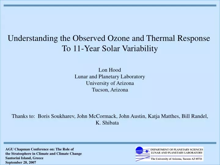
Understanding the Observed Ozone and Thermal Response To 11-Year Solar Variability Lon Hood Lunar and Planetary Laboratory University of Arizona Tucson, Arizona Thanks to: Boris Soukharev, John McCormack, John Austin, Katja Matthes, Bill Randel, K. Shibata.

E N D
Understanding the Observed Ozone and Thermal Response To 11-Year Solar Variability Lon Hood Lunar and Planetary Laboratory University of Arizona Tucson, Arizona Thanks to: Boris Soukharev, John McCormack, John Austin, Katja Matthes, Bill Randel, K. Shibata AGU Chapman Conference on: The Role of the Stratosphere in Climate and Climate Change Santorini Island, Greece September 28, 2007
MOTIVATION: 1. One potential sun-climate mechanism involves a dynamical response to stratospheric heating changes associated with increased solar UV radiation and solar-induced changes in stratospheric ozone (e.g., previous talk). 2. In order to simulate accurately the solar UV induced heating changes in the stratosphere, it is first necessary to determine and understand solar induced changes in the ozone distribution. It is also necessary to evaluate whether solar induced dynamical heating changes occur in the lower stratosphere (Kodera’s talk yesterday).
Evidence for a solar cycle variation of total ozone in the Version 8 TOMS/SBUV data record calibrated by Frith et al. (2004).
MULTIPLE REGRESSION STATISTICAL MODEL: , O3(t) = ctrendt + cQBOu30mb(t-lagQBO) + cvolcanicAerosol(t) + csolarMgII(t) + (t) where: , O3(t) = deviation of ozone from the seasonal mean t = time measured in 3-month seasonal increments u30mb(t- lagQBO) = FUB 30 hPa equatorial zonal wind speed (lagged) Aerosol(t) = Volcanic aerosol index (10 hPa and below only) MgII(t) = Solar MgII UV index (t) = residual error term
Ozone solar regression coefficient derived from V. 8 SBUV/SBUV(/2) Data: Shaded areas are statistically significant at 95% confidence.
Ozone solar regression coefficient derived from SAGE II Data: Shaded areas are statistically significant at 95% confidence.
Ozone solar regression coefficient derived from UARS HALOE Data: Shaded areas are statistically significant at 95% confidence.
Summary: Ozone solar cycle regression coefficient derived from three independent satellite data sets : SBUV Shaded areas are statistically significant at 95% confidence.
Ozone Solar Regression Coefficient (min to max) at low latitudes derived from SBUV, SAGE II, and UARS HALOE data: ? ? ??
Ozone Solar Regression Coefficient at low latitudes derived from SBUV data for three different time periods:
Comparison with Representative 2D and 3D Model Simulations: 25oS to 25oN
Comparison with Representative 2D and 3D Model Simulations: 25oS to 25oN
Austin et al. , ACP, 2007: Coupled Chemistry Climate Model Simulations of the Stratospheric O3 Variation (no QBO): 45-Year Simulations using observed SSTs, observed aerosol extinctions, and solar UV forcing (both 11-year and 27-day).
Matthes et al., in preparation, 2007: NCAR WACCM3: SAGE II: 110-Year Simulation relaxing to observed QBO winds, fixed SST’s, solar UV forcing, and particle precipitation forcing at high latitudes.
Possible Dynamical Mechanisms for Explaining the Unexpected Vertical Structure of the Solar Cycle Ozone Response in the Tropics: 1. Solar ultraviolet forcing effectively reduces the tropical upwelling rate near and approaching solar maxima (Kodera and Kuroda, 2002).
ERA-40 Seasonal Zonal Wind Solar Regression Coefficient 1979-2001 Crooks and Gray [2005] • Light shaded areas are significant at the 2 (95% confidence) level; dark shaded areas are significant at 99% confidence
Kodera and Kuroda (2002): Transport-induced ozone increase
Excluding periods following major volcanic eruptions, the decadal variation seen in the TOMS/SBUV column ozone record is also seen in the MSU Channel 4 temperature record at low latitudes.
Temperature solar regression coefficient derived from SSU/MSU4 Data (1979-2005) (K / 100 Units F10.7 ?) Courtesy of W. Randel
Crooks and Gray (2005): Temperature solar regression coefficient derived from ERA-40 Data (1979-2001) (Solar Max - Min) 1.75 K 0.5 Multiple regression model: Linear trend, QBO (first 2 PC’s of residual of a regression of ERA-40 zonal wind onto 18 other indices), solar cycle, volcanic aerosol, ENSO.
K. Shibata et al. (2007): Temperature solar regression coefficient derived from ERA-40 Data (1979-2001) 1.4 Multiple regression model: Linear trend, QBO (50 and 20 hPa eq. zonal wind time series), solar cycle, Pinatubo aerosol with lag, El Chichon aerosol with lag, ENSO.
The vertical structure of the temperature solar cycle variation estimated by Shibata et al. from the ERA-40 data is similar to that derived from long-term ozone data sets.
Possible Dynamical Mechanisms for Explaining the Unexpected Vertical Structure of the Solar Cycle Ozone Response in the Tropics: 1. Solar ultraviolet forcing effectively reduces the tropical upwelling rate near and approaching solar maxima (Kodera and Kuroda, 2002). 2. Solar induced circulation anomalies in the upper stratosphere may also perturb the equatorial quasi-biennial wind oscillation, which is the dominant cause of interannual ozone variability in the tropical lower stratosphere.
Possible Evidence for a Solar Cycle Modulation of the QBO as Proposed Originally by Salby and Callaghan (2000): R = -0.20 at zero lag; not significant. R = -0.51 at 1-year lag; significant at > 90% confidence. R = -0.64 at 2-year lag; significant at > 95% confidence.
During the east phase of the QBO (at 40 hPa), the vertical wind shear near 10 hPa is westerly. This produces transport-induced increases in NOx which cause photochemical ozone decreases. These decreases appear to be deeper and longer near solar maxima. East Phase Winds, ERA-40 Composite: E E From Pascoe et al., 2005
McCormack et al. , in press, 2007: 2D Model Simulations of the Effect on Ozone of a Solar-Modulated QBO: Exp 1: Solar UV Forcing Only (no QBO) Exp 2: Solar UV + Solar-Modulated QBO Exp 3: Solar UV + QBO + Imposed 11-Year Planetary Wave Forcing
CONCLUSIONS 1. A solar cycle variation of ozone and temperature occurs in the lower stratosphere. This may be caused by solar UV-induced changes in the subtropical winter upper stratosphere, which effectively reduces the tropical upwelling rate near solar maxima (Kodera and Kuroda, 2002). 2. No statistically significant solar cycle ozone response occurs in the tropical middle stratosphere (~ 10 hPa). It is suggested that this may be caused, at least in part, by a solar modulated QBO, which effectively enhances the odd nitrogen response to the easterly QBO phase under solar maximum conditions. 3. Several recent studies using CCCM’s have been able to simulate, at least qualitatively, the observed double-peaked structure of the tropical ozone response. However, to do so, it has so far been necessary to force the models using either observed SST’s or observed QBO winds. No fully self-consistent simulation has yet been performed.
During the east phase of the QBO (at 40 hPa), the vertical wind shear near 10 hPa is westerly. This produces transport-induced increases in NOx which cause photochemical ozone decreases. These decreases appear to be deeper and longer near solar maxima. East Phase Winds, ERA-40 Composite: E E From Pascoe et al., 2005
Evidence for a solar cycle variation of total ozone in the Version 8 TOMS/SBUV data record calibrated by Frith et al. (2004).
The UARS HALOE data set (e.g., Remsberg et al., JGR, 2001) provides relatively accurate measurements of the ozone profile in the lower stratosphere. HALOE
Correlation coefficient between TOMS/SBUV total ozone and HALOE ozone profile data averaged between 35S and 35N.
Excluding periods following major volcanic eruptions, the decadal variation seen in the TOMS/SBUV column ozone record is also seen in the MSU Channel 4 temperature record at low latitudes.
Two Possible Ways in Which the QBO may be Perturbed by the Solar Cycle: 1. McCormack, 2003; McCormack et al., 2007: Solar-induced heating changes modify the residual meridional circulation in the tropical stratosphere, producing vertical velocity anomalies causing the westerly QBO phase to descend more rapidly near solar maxima than near solar minima. This results in a longer westerly phase duration near solar minima. 2.Pascoe et al., 2005: The transition from the QBO west phase to the QBO east phase is inhibited when the tropical ascending branch of the Brewer-Dobson circulation is strong (Kinnersley and Pawson, JAS, 1996). The tropical ascending branch of the Brewer-Dobson circulation is strongest under solar minimum conditions (Kodera and Kuroda, 2002). Therefore, the duration of the westerly QBO phase tends to be longer under solar minimum conditions.
In the SAGE II data, there also appear to be deeper, longer ozone minima during the QBO east phase near the two solar maxima (excluding the Pinatubo period): E E E
Vertical structure of the ozone QBO: Randel and Wu, JAS, 1996 Vertical structure of the NOx QBO: Randel and Wu, JAS, 1996
Paper by Pascoe et al., JGR, 2005 (see also Baldwin et al., Rev. Geophys., 2001): 1. The rate of descent of the easterly QBO shear zone is slower and more variable than that of the westerly shear zone. Easterlies Westerlies From Baldwin et al., 2001 2. Kinnersley and Pawson (JAS, 1996) argue that changes in the descent rate of the QBO easterlies are influenced by the annual variation of the strength of the Brewer-Dobson upwelling at the equator, which is weakest during May, June, and July. Frequency of transitions from west to east phase at 44 hPa: From Pascoe et al., 2005
Paper by Pascoe et al., JGR, 2005: 3. Under solar maximum conditions, the rate of descent of easterlies is faster than otherwise. This causes the duration of the westerly phase to be longer under solar minimum conditions (cf. Salby and Callaghan, 2000). Easterly Descent Rate West Phase Duration at 44 hPa If the Kinnersley and Pawson interpretation is correct, this suggests a weaker B-D ascent branch under solar maximum conditions. The latter would be consistent with higher total ozone in the tropical lower stratosphere near solar maximum.
Dobson Data Evidence for a solar cycle variation of total ozone in ground-based Dobson spectrophotometer data (after WMO, 2006). (Anthropogenic Chlorine)
F10.7 Comparison of five long-term total ozone data sets with the solar 10.7 cm radio flux, a proxy for solar UV variations (from WMO, 2006).
Indirect evidence for a statistically significant response of tropical lower stratospheric ozone to 27-day solar UV variations. The observed column ozone response amplitude (about 0.9 DU / 0.01 Mg II units) is about 1.5 times larger than expected based on the observed upper and middle stratospheric ozone response.
Evidence for a statistically significant response of tropical lower stratospheric temperature to 27-day solar UV variations: NCEP Temperature, 20oS to 20oN: From Hood, GRL, 2003
First, consider a region where the solar signal is relatively strong and significant: 4 hPa, 20S - 40S