Exemplar Analysis

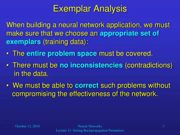
1. Exemplar Analysis • When building a neural network application, we must make sure that we choose an appropriate set of exemplars (training data): • The entire problem space must be covered. • There must be no inconsistencies (contradictions) in the data. • We must be able to correct such problems without compromising the effectiveness of the network. Neural Networks Lecture 11: Setting Backpropagation Parameters

2. Ensuring Coverage • For many applications, we do not just want our network to classify any kind of possible input. • Instead, we want our network to recognize whether an input belongs to any of the given classes or it is “garbage” that cannot be classified. • To achieve this, we train our network with both “classifiable” and “garbage” data (null patterns). • For the the null patterns, the network is supposed to produce a zero output, or a designated “null neuron” is activated. Neural Networks Lecture 11: Setting Backpropagation Parameters

3. Ensuring Coverage • In many cases, we use a 1:1 ratio for this training, that is, we use as many null patterns as there are actual data samples. • We have to make sure that all of these exemplars taken together cover the entire input space. • If it is certain that the network will never be presented with “garbage” data, then we do not need to use null patterns for training. Neural Networks Lecture 11: Setting Backpropagation Parameters

4. Ensuring Consistency • Sometimes there may be conflicting exemplars in our training set. • A conflict occurs when two or more identical input patterns are associated with different outputs. • Why is this problematic? Neural Networks Lecture 11: Setting Backpropagation Parameters

5. Ensuring Consistency • Assume a BPN with a training set including the exemplars (a, b) and (a, c). • Whenever the exemplar (a, b) is chosen, the network adjust its weights to present an output for a that is closer to b. • Whenever (a, c) is chosen, the network changes its weights for an output closer to c, thereby “unlearning” the adaptation for (a, b). • In the end, the network will associate input a with an output that is “between” b and c, but is neither exactly b or c, so the network error caused by these exemplars will not decrease. • For many applications, this is undesirable. Neural Networks Lecture 11: Setting Backpropagation Parameters

6. Ensuring Consistency • To identify such conflicts, we can apply a search algorithm to our set of exemplars. • How can we resolve an identified conflict? • Of course, the easiest way is to eliminate the conflicting exemplars from the training set. • However, this reduces the amount of training data that is given to the network. • Eliminating exemplars is the best way to go if it is found that these exemplars represent invalid data, for example, inaccurate measurements. • In general, however, other methods of conflict resolution are preferable. Neural Networks Lecture 11: Setting Backpropagation Parameters

7. Ensuring Consistency • Another method combines the conflicting patterns. • For example, if we have exemplars • (0011, 0101),(0011, 0010), • we can replace them with the following single exemplar: • (0011, 0111). • The way we compute the output vector of the new exemplar based on the two original output vectors depends on the current task. • It should be the value that is most “similar” (in terms of the external interpretation) to the original two values. Neural Networks Lecture 11: Setting Backpropagation Parameters

8. Ensuring Consistency • Alternatively, we can alter the representation scheme. • Let us assume that the conflicting measurements were taken at different times or places. • In that case, we can just expandall the input vectors, and the additional values specify the time or place of measurement. • For example, the exemplars • (0011, 0101),(0011, 0010) • could be replaced by the following ones: • (100011, 0101),(010011, 0010). Neural Networks Lecture 11: Setting Backpropagation Parameters

9. Ensuring Consistency • One advantage of altering the representation scheme is that this method cannot create any new conflicts. • Expanding the input vectors cannot make two or more of them identical if they were not identical before. Neural Networks Lecture 11: Setting Backpropagation Parameters

10. Training and Performance Evaluation • How many samples should be used for training? • Heuristic: At least 5-10 times as many samples as there are weights in the network. • Formula (Baum & Haussler, 1989): • P is the number of samples, |W| is the number of weights to be trained, and a is the desired accuracy (e.g., proportion of correctly classified samples). Neural Networks Lecture 11: Setting Backpropagation Parameters

11. Training and Performance Evaluation • What learning rate  should we choose? • The problems that arise when  is too small or to big are similar to the Adaline. • Unfortunately, the optimal value of  entirely depends on the application. • Values between 0.1 and 0.9 are typical for most applications. • Often,  is initially set to a large value and is decreased during the learning process. • Leads to better convergence of learning, also decreases likelihood of “getting stuck” in local error minimum at early learning stage. Neural Networks Lecture 11: Setting Backpropagation Parameters

12. Training and Performance Evaluation • When training a BPN, what is the acceptable error, i.e., when do we stop the training? • The minimum error that can be achieved does not only depend on the network parameters, but also on the specific training set. • Thus, for some applications the minimum error will be higher than for others. Neural Networks Lecture 11: Setting Backpropagation Parameters

13. Training and Performance Evaluation • An insightful way of performance evaluation is partial-set training. • The idea is to split the available data into two sets – the training set and the test set. • The network’s performance on the second set indicates how well the network has actually learned the desired mapping. • We should expect the network to interpolate, but not extrapolate. • Therefore, this test also evaluates our choice of training samples. Neural Networks Lecture 11: Setting Backpropagation Parameters

14. Training and Performance Evaluation • If the test set only contains one exemplar, this type of training is called “hold-one-out” training. • It is to be performed sequentially for every individual exemplar. • This, of course, is a very time-consuming process. • For example, if we have 1,000 exemplars and want to perform 100 epochs of training, this procedure involves 1,000999100 = 99,900,000 training steps. • Partial-set training with a 700-300 split would only require 70,000 training steps. • On the positive side, the advantage of hold-one-out training is that all available exemplars (except one) are use for training, which might lead to better network performance. Neural Networks Lecture 11: Setting Backpropagation Parameters

15. Example I: Predicting the Weather • Let us study an interesting neural network application. • Its purpose is to predict the local weather based on a set of current weather data: • temperature (degrees Celsius) • atmospheric pressure (inches of mercury) • relative humidity (percentage of saturation) • wind speed (kilometers per hour) • wind direction (N, NE, E, SE, S, SW, W, or NW) • cloud cover (0 = clear … 9 = total overcast) • weather condition (rain, hail, thunderstorm, …) Neural Networks Lecture 11: Setting Backpropagation Parameters

16. 100 km Example I: Predicting the Weather • We assume that we have access to the same data from several surrounding weather stations. • There are eight such stations that surround our position in the following way: Neural Networks Lecture 11: Setting Backpropagation Parameters

17. Example I: Predicting the Weather • How should we format the input patterns? • We need to represent the current weather conditions by an input vector whose elements range in magnitude between zero and one. • When we inspect the raw data, we find that there are two types of data that we have to account for: • Scaled, continuously variable values • n-ary representations of category values Neural Networks Lecture 11: Setting Backpropagation Parameters

18. Example I: Predicting the Weather • The following data can be scaled: • temperature (-10… 40 degrees Celsius) • atmospheric pressure (26… 34 inches of mercury) • relative humidity (0… 100 percent) • wind speed (0… 250 km/h) • cloud cover (0… 9) • We can just scale each of these values so that its lower limit is mapped to some and its upper value is mapped to (1 - ). • These numbers will be the components of the input vector. Neural Networks Lecture 11: Setting Backpropagation Parameters

19. Example I: Predicting the Weather • Usually, wind speeds vary between 0 and 40 km/h. • By scaling wind speed between 0 and 250 km/h, we can account for all possible wind speeds, but usually only make use of a small fraction of the scale. • Therefore, only the most extreme wind speeds will exert a substantial effect on the weather prediction. • Consequently, we will use two scaled input values: • wind speed ranging from 0 to 40 km/h • wind speed ranging from 40 to 250 km/h Neural Networks Lecture 11: Setting Backpropagation Parameters

20. Example I: Predicting the Weather • How about the non-scalable weather data? • Wind direction is represented by an eight- component vector, where only one element (or possibly two adjacent ones) is active, indicating one out of eight wind directions. • The subjective weather condition is represented by a nine-component vector with at least one, and possibly more, active elements. • With this scheme, we can encode the current conditions at a given weather station with 23 vector components: • one for each of the four scaled parameters • two for wind speed • eight for wind direction • nine for the subjective weather condition Neural Networks Lecture 11: Setting Backpropagation Parameters

21. … … … our station north northwest Example I: Predicting the Weather • Since the input does not only include our station, but also the eight surrounding ones, the input layer of the network looks like this: … The network has 207 input neurons, which accept 207-component input vectors. Neural Networks Lecture 11: Setting Backpropagation Parameters

22. Example I: Predicting the Weather • What should the output patterns look like? • We want the network to produce a set of indicators that we can interpret as a prediction of the weather in 24 hours from now. • In analogy to the weather forecast on the evening news, we decide to demand the following four indicators: • a temperature prediction • a prediction of the chance of precipitation occurring • an indication of the expected cloud cover • a storm indicator (extreme conditions warning) Neural Networks Lecture 11: Setting Backpropagation Parameters

23. Example I: Predicting the Weather • Each of these four indicators can be represented by one scaled output value: • temperature (-10… 40 degrees Celsius) • chance of precipitation (0%… 100%) • cloud cover (0… 9) • storm warning: two possibilities: • 0: no storm warning; 1: storm warning • probability of serious storm (0%… 100%) • Of course, the actual network outputs range from to (1 - ), and after their computation, if necessary, they are scaled to match the ranges specified above. Neural Networks Lecture 11: Setting Backpropagation Parameters