Download
1 / 62
670 likes | 1.24k Views
Fluid Simulation for Computer Animation. Greg Turk College of Computing and GVU Center Georgia Institute of Technology. Why Simulate Fluids?. Feature film special effects Computer games Medicine (e.g. blood flow in heart) Because it’s fun. Fluid Simulation.

E N D
Fluid Simulation forComputer Animation Greg Turk College of Computing and GVU Center Georgia Institute of Technology
Why Simulate Fluids? • Feature film special effects • Computer games • Medicine (e.g. blood flow in heart) • Because it’s fun
Fluid Simulation • Called Computational Fluid Dynamics (CFD) • Many approaches from math and engineering • Graphics favors finite differences • Jos Stam introduced fast and stable methods to graphics [Stam 1999]
Diffusion Pressure Advection Body Forces Change in Velocity Navier-Stokes Equations u=0 ut= k2u –(u)u – p + f Incompressibility
Navier-Stokes Equations u=0 ut= k2u–(u)u – p + f Incompressibility Diffusion Pressure Advection Body Forces Change in Velocity
Finite Differences Grids • All values live on regular grids • Need scalar and vector fields • Scalar fields: amount of smoke or dye • Vector fields: fluid velocity • Subtract adjacent quantities to approximate derivatives
Scalar Field (Smoke, Dye) … 5.1 1.2 3.7 cij
Diffusion cij
1 1 -4 1 1 change in value value relative to neighbors Diffusion ct = k2c cijnew = cij + k Dt (ci-1j + ci+1j + cij-1 + cij+1 - 4cij)
More Diffusion Some Diffusion Original Diffusion = Blurring
Vector Fields (Fluid Velocity) uij = (ux,uy)
viscosity Two separate diffusions: uxt= k2ux uyt= k2uy Vector Field Diffusion ut= k2u … blur the x-velocity and the y-velocity
Effect of Viscosity Low Medium High Very High • Each one is ten times higher viscosity than the last “Melting and Flowing” Mark Carlson, Peter J. Mucha, Greg Turk Symposium on Computer Animation 2002
Variable Viscosity • Viscosity can vary based on position • Viscosity field k can change with temperature • Need implicit solver for high viscosity
Navier-Stokes Equations u=0 ut= k2u –(u)u – p + f Incompressibility Diffusion Pressure Advection Body Forces Change in Velocity
Advection 0.3 2.7 0.3
change in value advection current values Scalar Field Advection ct=–(u)c
Two separate advections: uxt=–(u)ux uyt=–(u)uy Vector Field Advection ut=–(u)u … push around x-velocity and y-velocity
Advection • Easy to code • Method stable even at large time steps • Problem: numerical inaccuracy diffuses flow
Diffusion/dissipation in first order advection After 360 degree rotation using first order advection Original Image
Solution: BFECC 1) Perform forward advection 2) Do backward advection from new position 3) Compute error and take correction step 4) Do forward advection from corrected position “Flowfixer: Using BFECC for Fluid Simulation” ByungMoon Kim, Yingjie Liu, Ignacio Llamas, Jarek Rossignac Eurographics Workshop on Natural Phenomena 2005
Forward Compensate Forward Backward error Intuition to BFECC
Navier-Stokes Equations u=0 ut= k2u –(u)u– p + f Incompressibility Diffusion Pressure Advection Body Forces Change in Velocity
Low divergence Zero divergence Divergence High divergence
Enforcing Incompressibility • First do velocity diffusion and advection • Find “closest” vector field that is divergence-free • Need to calculate divergence • Need to find and use pressure
uyij+1 ? -uxi-1j uxi+1j -uyij-1 Measuring Divergence u=? uij=(uxi+1j - uxi-1j) + (uyij+1-uyij-1)
zero Pressure Term unew= u – p Take divergence of both sides… unew= u – p u = 2p
1 known unknown 1 1 -4 1 Pressure Term u = 2p pnew = p + e( u - 2p) Let dij = uij pnewij = pij + e(dij - (pi-1j + pi+1j + pij-1 + pij+1 - 4pij))
Pressure Term unew= u – p …and velocity is now divergence-free Found “nearest” divergence-free vector field to original.
Fluid Simulator Diffuse velocity Advect velocity Add body forces (e.g. gravity) Pressure projection Diffuse dye/smoke Advect dye/smoke
“Real-Time Fluid Dynamics for Games” Jos Stam, March 2003 (CDROM link is to source code) www.dgp.toronto.edu/people/stam/reality/Research/pubs.html
Rigid Objects • Want rigid objects in fluid • Use approach similar to pressure projection “Rigid Fluid: Animating the Interplay Between Rigid Bodies and Fluid” Mark Carlson, Peter J. Mucha and Greg Turk Siggraph 2004
Rigid Fluid Method 1) Solve Navier-Stokes on entire grid, treating solids exactly as if they were fluid 2) Calculate forces from collisions and relative density 3) Enforce rigid motion for cells inside rigid bodies
Small-scale liquid-solid Interactions What makes large water and small water behave differently? Surface Tension (water: 72 dynes/cm at 25º C) Viscosity (water: 1.002 x 10⁻³ N·s/m2 at 20º C) Lake ( >1 meter) Water drops (millimeters)
Surface Tension Normal (always pointing outward) Surface Tension Force
Water/Surface Contact hydrophillic hydrophobic
Virtual Liquid Virtual Surface Virtual Surface Method Air Liquid Solid
Air Liquid Virtual Liquid Solid Virtual Surface Advancing to right:qc>qs Virtual Surface Method 1) Creating a virtual surface 2) Estimate curvature from new fluid surface 3) Kink will “push” the fluid towards stable contact angle
Air Virtual Liquid Solid Virtual Surface Receding to left:qc<qs Virtual Surface Method 1) Creating a virtual surface 2) Estimate curvature from new fluid surface 3) Kink will “push” the fluid towards stable contact angle