Download
1 / 23
230 likes | 388 Views
Counting Graph Colourings by using Sequences of Subgraphs. Charilaos Efthymiou DIMAP University of Warwick DIMAP Summer School – July 2010. Counting. Problem : Given Find the cardinality of the set of feasible solutions

E N D
Counting Graph Colourings by using Sequences of Subgraphs Charilaos Efthymiou DIMAP University of Warwick DIMAP Summer School – July 2010
Counting • Problem: Given Find the cardinality of the set of feasible solutions • Examples: matching, independent sets, proper colourings, bin packing, SAT
Graph Colouring G=(V, E) Set of colours{1,…,k} (Proper) Colouring σ:V →{1,…,k} and σ(v)≠σ(u)for every {v,u}E 1 1 2 1 1 3 Colours :{1, 2, 3, 4} 6 3 2 4 3 5
Counting Vs Sampling G=(V, E) 2 1 Set of colours{1,…,k} c d Z(G, k): k-colouring of G a 3 e Process: Choose u.a.r. a k-colouring of the graph b 6 Ei,j: “Vertices i, j receive different colour” 4 5 pa:: Pr[ E1,6 in Ga] pb: Pr[ E1,4 in Gb] pc: Pr[ E2,6 in Gc] pd: Pr[ E2,5 in Gd] pe: Pr[ {6,3} in Ge] Z(G,k)=|V|k papbpcpdpe
Counting • Exact counting is hard, • Valiant ‘79P class • Approximate counting using Rapidly Mixing Markov Chains • Celebrated achievements: FPRAS for • Permanents: Jerrum, Sinclair 1989, Jerrum Sinclair Vigoda 2001 • Volume of convex body: Dyer, Frieze Kannan 1991 • Counting independent sets in degree-4 graphs: Luby and Vigoda 1997
Graph k-colourings • Maximum degree Δ • [Vigoda 99] k>11/6Δ– arbitrarygraph • [Mοssel & Sly 08] Random graphs with fixed expected degree d , with k>f(d) • [Hayes, Vera & Vigoda] Planar Graphs k> Ω(Δ/log Δ)
For this talk… • We propose algorithms which are not based on Markov Chains. • Compute the corresponding probabilities directly. • Weakness: • We only compute ε-approximation to log Z(G, k) • Strength: • Deterministic • Explicit results for Gnp
Works for Det. Counting • Colourings • Regular graphs with high girth Δ+1-colours- PTAS • Bandyopadhyay, Gamarnik 2005 • G with girth 4, 2.8Δ-colours FPTAS • Gamarnik, Katz 2007 • Sparse Random Graphs with number of colours that depend on the expected degree -PTAS • Efthymiou, Spirakis 2008. • Graph matchings - FPTAS • Bayatui, Gamarnik, Katz, Nair, Tetali 2007. • Independent sets FPTAS • Weitz 2006
Easy Examples… • Trees • Compute each probability recursively! • DP - - For constant k the time-complexity is O(n) • Graphs of bounded treewidth • Graphs with number of k-colourings (proper & non-proper) that is O(nc)
Efficient computation of marginals – Correlation decay u v A B C t
3-step algorithm • Compute Pr[Euv] on the “small” graph. • Prove independence from boundary conditions. • Dobrushin’s Condition for Uniqueness of Gibbs measure • Project to the initial graph.
Reduce computational load differently… l1 r1 u l2 r2 v l3 r3 l4 r4 t A B C
Reduce computational load differently… l1 r1 u l2 r2 v l3 r3 l4 r4 A B C
Implications on spatial mixing conditions l1 r1 u l2 r2 v l3 r3 l4 r4 A B C t t L(l3, t): Vertices outside red cycle L(r3, t): Vertices outside green cycle
Comparison with the first approach l1 r1 u l2 r2 v l3 r3 l4 r4 t L(l3, t): Vertices outside red cycle
Theorem - Accuracy l1 r1 u l2 r2 v l3 r3 l4 r4
Spatial Correlation decay G=(V,E) u BP(v,u) Product measure: Pq Pr[Disagreeing]=q Pr[Non-Disagreeing]=1-q “Path of disagreement between u & v” v
Applications I – Sparse Gnp • The underlying graph is Gnp with expected degree d, d is fixed • Vertex set V={1,…, n} • Each possible edge appear with probability p, independently of the others. • Expected degree is d is fixed real, i.e. p=d/n • The maximum degree is Θ(log n/ loglog n) • Chromatic number Constant
Applications I – Sparse Gnp • Isolate Θ(log n) neighborhoods around u,v • Tree with additional Θ(log n) edges • Computations by Dynamic Programming • Using k≥(2+ε)d with probability 1-n-Ω(1) we get a polynomial time, n-Ω(1)-approximation of log Z(Gnp,k).
Applications II – Locally α-dense graphs • G(V,E) is locally α-denseof bounded maximum degree Δ if • For all {w1, w2} E w2 has at most (1-α)Δ neighbors which are not adjacent to w1 • α [0,1] is a parameter of the model
Applications II – Locally dense graphs • For k>(2-α)Δ we get a (log n)-Ω(1)-approximation of log Z(G,k), in polynomial time. • If, additionally, every Θ(log n) neighborhood of G has constant treewidth, then we get a n-Ω(1)-approximation of log Z(G,k), in polynomial time.