Download

1 / 15
180 likes | 513 Views
Data Envelopment Analysis (DEA) Tool for Benchmarking. DEA is a key benchmarking tool - Multidimensional analytical in nature - Deals with multiple-input, multiple-output productivity ratios.

E N D
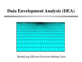
Data Envelopment Analysis (DEA) Tool for Benchmarking
DEA is a key benchmarking tool - Multidimensional analytical in nature - Deals with multiple-input, multiple-output productivity ratios • It supports the identification of Best Practice Units and can help identify those that either need improvement or could be used for benchmarking. • Could be deployed in Internal, Process, Competitive and Strategic Benchmarking. • Offers more insight than a traditional “gap analysis” generally used in benchmarking. • Basic intuition: • - Input/output model formulation that defines the efficiencies of various entities called DMU’s, the decision making units; • - The analytics discriminates the relative efficiencies of various DMU’s; • - Identifies Peers for the inefficient firms, whom they can emulate in order to improve their efficiencies.
Which Unit is most productive?(one input and one output) DMU labor hrs. #cust. 1 100 150 2 75 140 3 120 160 4 100 140 5 40 50 DMU = decision making unit
DMU labor hrs. #cust. #cust/hr Relative Efficiency 1 100 150 1.50 80.21% 2 75 140 1.87 100 % 3 120 160 1.33 71.12% 4 100 140 1.40 74.87% 5 40 50 1.25 66.84% #cust. 200 x slope = 1.87 x x x 100 DMU’s 1,3,4,5 are dominated by DMU 2. x labor hrs. 50 100
PERFORMANCE DATA OF FOUR DMUs (two inputs and one output)
COMPARITIVE PERFORMANCE OF FOUR DMUs COMPARITIVE PERFORMANCE OF FOUR DMUs
B A D (8.5, 11) (1.0, 4.78) (3.0, 7.70) Efficiency Frontier C (.93, 5.57) Capital employed / Value Added Efficiency Frontier O Employee / Value Added
B A D E (8.5, 11) (1.0, 4.78) (3.0, 7.70) (3.69, 4.78) Efficiency Frontier C (.93, 5.57) Capital employed / Value Added Efficiency Frontier O Employee / Value Added
E B A D (3.69, 4.78) (8.5, 11) (1.0, 4.78) (3.0, 7.70) Efficiency Frontier C (.93, 5.57) Capital employed / Value Added Efficiency Frontier Best PossiblePerformance Relative Eff. = ActualPerformance √(3.692+4.782) OB = = = 43.44% √(8.52+112) OE O Employee / Value Added
D E B F A (8.5, 11) (3.69, 4.78) (.93, 11) (1.0, 4.78) (3.0, 7.70) Efficiency Frontier C (.93, 5.57) Capital employed / Value Added Efficiency Frontier O Employee / Value Added
A F G D B E (8.5, 11) (.93, 11) (3.69, 4.78) (3.0, 7.70) (8.5, 4.78) (1.0, 4.78) Efficiency Frontier C (.93, 5.57) Capital employed / Value Added Efficiency Frontier O Employee / Value Added
E F G A B D (3.69, 4.78) (8.5, 4.78) (1.0, 4.78) (8.5, 11) (.93, 11) (3.0, 7.70) Efficiency Frontier C (.93, 5.57) Capital employed / Value Added Efficiency Frontier Best PossiblePerformance Relative Eff. = ActualPerformance √(3.692+4.782) OB = = = 43.44% √(8.52+112) OE O Employee / Value Added
Setting Performance Targets for the Inefficient Firms • Firm B can move up to the efficient frontier in at least three ways: • Reducing only the number of employees: • By moving to the point F • => Input Target for Employees = 0.2 x 0.93 = 0.186 • => Employees Surplus = Current input – Input target • = 1.7 – 0.186 = 1.514 • 2. Reducing only its capital employed: • By moving to point G • => Input Target for Capital = 0.2 x 4.78 = 0.956 • => Capital Surplus = Current input – Input target • =2.000 – 0.956 = 1.244 • 3. (a) Reducing both, the capital employed as well as the number of employees, in the same ratio; or • (b) Enhancing value added only; • By moving to point E