Download
1 / 24
250 likes | 762 Views
Atmospheric boundary layers and turbulence II. Wind loading and structural response Lecture 7 Dr. J.D. Holmes. Atmospheric boundary layers and turbulence. Topics : . Turbulence (Section 3.3 in book) - gust factors, spectra, correlations. Effect of topography (Section 3.4 in book).

E N D
Atmospheric boundary layers and turbulence II Wind loading and structural response Lecture 7 Dr. J.D. Holmes
Atmospheric boundary layers and turbulence • Topics : • Turbulence (Section 3.3 in book) - gust factors,spectra, correlations • Effect of topography (Section 3.4 in book) • Change of terrain (Section 3.5 in book)
T=10 min. Atmospheric boundary layers and turbulence Gust speeds and gust factors : • The peak wind speed in a given time period (say 10 minutes) is a random variable The ‘expected value’ or average peak can be written as : where g is a peak factor, in this case equal to 3.5 From the response time of anemometers (Dines, cup) used for long-term wind measurements, measured peak gusts are often quoted as a ‘3 second gusts’
Atmospheric boundary layers and turbulence Gust speeds and gust factors : • Gust factor, G, is the ratio of the maximum gust speed to the mean wind speed : At 10 metres height in open country, G 1.45 ( higher latitude gales) In hurricanes, G 1.55 to 1.66
Atmospheric boundary layers and turbulence Wind spectra : As discussed in Lecture 5, the spectral density function provides a description of the frequency content of wind velocity fluctuations Empirical forms based on full scale measurements have been proposed for all 3 velocity components These are usually expressed in a non-dimensional form, e.g. : Sometimes u*2 orU2 is used in the denominator
Atmospheric boundary layers and turbulence Wind spectra : The most important turbulence component is the longitudinal component u(t). The most commonly used spectrum for u is known as the von Karman spectrum : lu is the integral scale of turbulence, which can also be obtained from the auto-correlation function (Lecture 5). U, u ,lu must be specified to numerically determine Su(n) Note that at high frequencies, n.Su(n) n-2/3, or Su(n) n-5/3
Atmospheric boundary layers and turbulence Wind spectra : von Karman spectrum : at zero frequencies, Su(0) 4 u2 lu /U at high frequencies, n.Su(n) n-2/3, or Su(n) n-5/3 The latter is a property of turbulence in a frequency range known as the inertial sub-range
Atmospheric boundary layers and turbulence Wind spectra : zero frequency limit : From Lecture 5 : since auto-correlation is a symmetrical function of : u(-) = u() setting n = 0 T1 is time scale (Lecture 5) (von Karman spectrum satisfies this)
von Karman 0.3 n.Su(n)/u2 0.2 0.1 0.0 0.01 0.10 1.00 10.00 n.lu / U Atmospheric boundary layers and turbulence von Karman spectrum : Maximum value of 0.271 occurs at n.lu/U of 0.146
Busch & Panofsky 0.3 n.Sw(n)/w2 0.2 0.1 0.0 0.01 0.10 1.00 10.00 n.z/ U Atmospheric boundary layers and turbulence Busch and Panofsky spectrum for vertical component w(t): Length scale in this case is height above ground, z Maximum value of 0.258 occurs at n.z/U of 0.30
Atmospheric boundary layers and turbulence Co-spectrum of longitudinal velocity component : As discussed in Lecture 5, the normalized co-spectrum represents a frequency-dependent correlation coefficient : It is important use is to determine the strength of wind forces at the natural frequency of a structure, and hence the resonant response Exponential decay function : As separation distance z increases, or frequency, n, decreases, co-spectrum (z,n) decreases Disadvantages : 1) goes to 1 as n0, even for very large z 2) does not allow negative values
Atmospheric boundary layers and turbulence Correlation of longitudinal velocity component : Covariance and cross-correlation coefficient were discussed in Lecture 5 The correlation properties for the longitudinal velocity components, at points with vertical or horizontal separation are important for wind loads on tall towers, buildings, transmission lines etc. Exponential decay function : uu exp [-Cz1 - z2] As separation distance z1 - z2 increases, correlation coefficient uu decreases
shallow escarpment shallow hill or ridge Atmospheric boundary layers and turbulence Effects of topography : Shallow topography : no separation of flow (follows contours) Predictable from computer models, wind-tunnel models
separation steep escarpment steep escarpment separation separation steep hill or ridge Atmospheric boundary layers and turbulence Effects of topography : Steep topography : separation of flow occurs Less predictable from computer models, wind-tunnel models OK at large enough scale
effective slope 0.3 Atmospheric boundary layers and turbulence Effects of topography : Effective upwind slope : about 0.3 (17 degrees) Upper limit on speed up effect as upwind slope increases
for mean wind speeds for peak gust wind speeds : Atmospheric boundary layers and turbulence Topographic multiplier : denoted by Mt :: Can be greater or less than 1. Codes only give values > 1 ASCE-7 : Kz,t = (1 + K1K2K3)2Mt = 1 + K1K2K3
crest H /2 Lu Atmospheric boundary layers and turbulence Shallow hills : k is a constant for a given type of topography s is a position factor = 1.0 at crest <1 upwind and downwind, and with increasing height is the upwind slope = H/2Lu
Atmospheric boundary layers and turbulence Shallow topography : k is a constant for a given type of topography (ridge, escarpment, hill) • 4.0 for two-dimensional ridges • 1.6 for two-dimensional escarpments • 3.2 for three-dimensional (axisymmetric) hills
Atmospheric boundary layers and turbulence Shallow topography : Gust multiplier : Assume that standard deviation of longitudinal turbulence, u, is unchanged as the wind flow passes over the hill
Atmospheric boundary layers and turbulence Steep topography : Can be treated approximately by taking an effective slope, ' = 0.3 then same formulae are used, i.e. : However these formulae are less accurate than those for shallow hills and do not account for separations at crest of escarpment or on lee side of a hill or ridge
z xi(z) inner boundary layer x roughness length zo2 roughness length zo1 Atmospheric boundary layers and turbulence Change of terrain : At a change of terrain roughness, adjustment takes place within an ‘inner boundary layer Within the inner boundary layer, the logarthmic law with the roughness length, z02, applies, but the wind speeds must match at the edge of the inner boundary layer Full adjustment of the magnitudes of the mean wind speeds does not occur until the inner boundary layer fills the entire atmospheric boundary layer - this could take as much as 50 km (30 miles) of the new terrain
Atmospheric boundary layers and turbulence Change of terrain : For flow from smooth to rougher terrain (z02 > z01) : (Deaves, 1981) For flow from rough to smoother terrain (z02 < z01) :
where and are the asymptotic gust velocities over fully-developed terrain of type 1 (upstream) and 2 (downstream). Atmospheric boundary layers and turbulence Change of terrain : Turbulence and gust wind speeds adjust faster than mean speeds to a change of terrain For gust speed at 10 metres, an exponential adjustment can be assumed : (Melbourne, 1992)