Download
1 / 21
210 likes | 369 Views
Software / Hardware Partitioning Techniques. SHaPES : A New Approach. Background. The allocation of a system’s functionality into hardware and software components has a significant impact on total system cost. Partitioning algorithms usually target one of the following types of systems:

E N D
Software / Hardware Partitioning Techniques SHaPES: A New Approach
Background • The allocation of a system’s functionality into hardware and software components has a significant impact on total system cost. • Partitioning algorithms usually target one of the following types of systems: • Single-processor, single-ASIC (or FPGA) SOC • Multiple processing element (PE), distributed heterogeneous system
Background • The three main sub-problems that must be solved when determining the hardware-software partitioning of a system: • Functional Clustering – cluster system functionality into a set of tasks • Allocation – allocate a task to either hardware or software • Scheduling – schedule tasks to ensure correct timing • These problems are independent
Background • These are hard problems! • Allocation and scheduling are NP-hard • There’s an exponential number of different possible clusters • Huh? • NP-hard means superpolynomial time (e.g. O(2^N)) • We’ll have to use a heuristics based approach if we want to get a solution in our lifetime
Background • Heuristic-based solutions have their own problems • Random Search: takes a long time • Iterative Improvement: quality of final solution proportional to quality of initial revision • Constructive: yields good solutions, good execution time, etc., but scheduling is a bi-product, not the main focus.
Who you gonna call? SHaPES “Software-Hardware Partitioning For Embedded Systems”
Formulating The Problem • This approach assumes a single microprocessor and single ASIC SOC as the target platform • Looks at the partitioning problem as a real-time scheduling problem… we’re scheduling a set of periodic and sporadic tasks • Tasks are implemented either completely in hardware or software
Formulating The Problem • Implementation Costs We Care About: • Hardware Area • Power Consumption • Timing Constraints • But, a scheduling problem can’t model size and power constraints!
Formulating The Problem • Hard-timing constraints modeled as follows: • Processing Time (pj): How long it takes a task to execute on the microprocessor uninterupted • Release Time (rj): The earliest moment as which a task can begin execution • Deadline (dj): The time by which the task should be completed • Weight (wj): The importance of a task
Formulating The Problem • Under this model, all tasks start out initially in software. Rejecting a task implies it should be implemented in hardware. • Since hardware is always assumed to be fast-enough for a task, you could cheat and reject all tasks, but that’s not realistic
Formulating The Problem • Violations are modeled as “costs;” the further past the deadline a task completes and the higher the weight of the task, the higher the penalty • Delegating a task to hardware is also modeled as a cost, called the “rejection cost,” represented by ej
Formulating The Problem • Thus, the crux of the problem is: Partition the set of tasks such that the sum of costs incurred by overtime software tasks and the rejection costs incurred by implementing a task in hardware are minimized
Formulating The Problem • But, sometimes a task has to wait around for other tasks to complete before they can start! • These dependencies are accounted for and are referred to as “precedence constraints” in the paper.
Solving The Scheduling Problem • Scheduling a set of jobs to minimize overall tardiness is an old problem (older than you) • Some simple approaches are: • Earliest Due Date (EDD) • Shortest Processing Time First (SPT) • This paper, however, uses ATC or Apparent Tardiness Cost
Solving The Scheduling Problem • Tasks are scheduled in non-increasing priority with priority defined as:
Solving The Scheduling Problem • Note that the formula includes the processing time of the subsequent task • Thus, that value is replaced with kp, where p is the average execution time, and k is a look-ahead factor whose value depends on how many tasks are completing late.
Solving The Scheduling Problem • ATC dispatching is basically a proportion of the weight to the execution time, scaled by how much time you still have to schedule the task • Thus, the priority of a task increases the closer you are to its deadline • Good News: The algorithm still works pretty well even if your processing time estimates contain errors (but that’s another paper)
Dealing With Idleness • Basic Idea: ATC designates a task that should be run next, but its release time has not yet been reached. The system will have to sit idle until that time is reached. • Solution: Scale the priority of a task proportional to this idleness:
Rubber Hits The Road • Start with all tasks initially in software partition • At a given time t, take the task with the largest ATC • Multiply its weight by its tardiness (completion time – deadline) • If the above cost is greater than its rejection cost, reject it to hardware and pick another task
Rubber Hits The Road • Repeat this until you have an ordered set of software tasks, and a set of tasks that have been rejected to hardware. • Re-run the algorithm for the hardware tasks with appropriate processing times. • If you have no rejected hardware tasks, you’re done! • If you do have rejected hardware tasks, you need to pick different hardware and start over.