Download

1 / 19
200 likes | 547 Views
Lattice Vibrations & Phonons B BW, Ch. 7 & YC, Ch 3. Lattice Dynamics or “Crystal Dynamics”. Lattice Dynamics A whole subfield of solid state physics! Most discussion will apply to any crystalline solids , not just semiconductors. A VERY OLD subfield!

E N D
Lattice Dynamics or “Crystal Dynamics” Lattice DynamicsA whole subfield of solid state physics! Most discussion will apply to any crystalline solids, not just semiconductors. • A VERY OLD subfield! • A “dead” subfield (no longer an area of active research!) • Recallback near the beginning of our bandstructure discussion. There, we had a many electron, many ion Hamiltonian(core electrons + nuclei = ions): H = He + Hi + He-i Electron Kinetic Energy + Interactions with Other Electrons Electron-Ion Interaction Ion Kinetic Energy + Interactions with Other Ions
Back to early in our bansdtructure discussion:Hamiltonian for a Perfect, Periodic CrystalNeelectrons, Niions; Ne, Ni ~ 1023 (huge!)Notation: i = electron; j = ion • The classical, many-body Hamiltonian is:(Gaussian units!) H = He + Hi + He-i He = Pure electronic energy = KE(e-) + PE(e- -e-) He= ∑i(pi)2/(2mi) + (½ )∑i∑i´[e2/|ri - ri´|] (i i´) Hi = Pure ion energy = KE(i) + PE(i-i) Hi= ∑j(Pj)2/(2Mj) + (½)∑j∑j´[ZjZj´ e2/|Rj - Rj´|] (j j´) He-i = Electron-ion interaction energy = PE(e--i) He-i= - ∑i∑j[Zje2/|ri - Rj|] Lower case r, p, m: Electron position, momentum, mass Upper case R, P, M: Ion position, momentum, mass
The Classical,many-bodyHamiltonian: H = He + Hi + He-i • We then focused on electronic properties calculations (bandstructures, etc.) & through some approximations, reduced this many electron Hamiltonian to a ONE ELECTRON HAMILTONIAN! • Now, instead, we will focus our attention on The Ion Motion Part ofH.
RecallThe Born-Oppenheimer(Adiabatic)Approximation • This is an approximation we made in order to reduce the electronic Hamiltonian to a 1 electron Hamiltonian. • Thisapproximation separates the electron & ion motion.A rigorous proof of the result requires detailed, many body Quantum Mechanics. • A Qualitative(semiquantitative)justification: • The ratio of the electron & ion masses: (me/Mi) ~ 10-3( << 1) or smaller! Classically, the massive ions movemuch slowerthan the very small mass electrons!
Typical ionic vibrational frequencies: υi ~ 1013 s-1 The time scale of the ion motion is: ti ~ 10-13 s • Electronic motion occurs at energies of about a bandgap: Eg= hυe = ħω~ 1 eV υe ~ 1015 s-1 te ~ 10-15 s • So, classically, the Electrons Respond to the Ion Motion ~ Instantaneously! As far as the electrons are concerned, the ions are ~ stationary! In the electron Hamiltonian, Hethe ions can be treated as stationary!
Born-Oppenheimer (Adiabatic) Approximation • Now, lets look at the Ions: The massive ions cannot follow the rapid, detailed electron motion. The Ions ~ see an Average Electron Potential. In the ion Hamiltonian,Hi , the electrons can be treated in an average way! (BW, Chapter 7, lattice vibrations)
ImplementationBorn-Oppenheimer(Adiabatic)Approximation • Write the coordinates for the vibrating ions as Rj = Rjo + δRj, Rjo = equilibrium ion position δRj= (small) deviation from equilibrium position • The many body electron-ion Hamiltonian is (schematic!): He-i ~ = He-i(ri,Rjo) + He-i(ri,δRj) • The New many body Hamiltonianin this approximation is: H = He(ri) + He-i(ri,Rjo) + Hi(Rj) + He-i (ri,δRj) (1) Neglect the last 2 terms in electron band calculations. Keep ONLY THEM for vibrational properties. or H= HE[1st 2 terms of (1)] + HI[2nd 2 terms of (1)] Here,HE = electron part(Gives the energy bands. Thoroughly discussed already!) HI = ion part (Gives the phonons, BW Ch. 7). We now focus on this part only.
Before we made theBorn-Oppenheimer Approximation, the Ion Hamiltonianwas: HI = Hi + He-i = j[(Pj)2/(2Mj)] + (½)jj´[ZjZj´e2/|Rj-Rj´|] -ij[Zje2/|ri-Rj|] • Because the ion ions are moving (lattice vibrations), the ion positions Rj are obviously time dependent. • After a tedious implementation of the Born-Oppenheimer Approximation, the Ion Hamiltonianbecomes: HI j[(Pj)2/(2Mj)] + Ee(R1,R2,R3,…RN) • Ee Average total energy for all ions at positions Rj (The average of the ion-ion interaction + electron-ion interaction) • A detailed Quantum Mechanical analysis (Born-Oppenheimer Approximation) results in the fact that Ee ground state total energy of the many electron problem as a function of all Rj • This results in the fact that Eeacts as an effective potential for the ion motion
The total electronic ground state energyEeacts as an effective potential energy for the ion motion. • Note that Ee depends on the electronic states of all e-AND the positions of all ions! To calculate it from first principles, the many electron problem must first be solved! • With modern computational techniques, it is possible to: 1. Calculate Ee to a high degree of accuracy (as a function of all Rj). 2. Then, use the calculated electronic structure of the solid tocompute & predict it’s vibrational properties. • This is a HUGE computational problem. With modern computers, this can be done & often is done. • But, historically, this was very difficult or even impossible to do. Therefore, people used many different empirical models instead.
Lattice Dynamics • Most work in this area was donelong beforethe existence of modern computers! • This is anOLDfield. It is also essentiallyDEADin the sense that little, if any, new research is being done. • The work that was done in this field relied on phenomenological (empirical), non-first principles, methods. • However,it is still useful to briefly look at these empirical models because doing so will (hopefully) teach us something about the physics of lattice vibrations.
Consider the coordinates of each vibrating ion: Rj Rjo + δRj Rjo equilibrium ion position δRj vibrational displacement amplitude • As long as the solid is far from it’s melting point, it is always true that |δRj| << a,where a lattice constant. If this were not true, the solid would melt or “fall apart”! • Lets use this fact to expand Eein a Taylor’s series about the equilibrium ion positions Rjo. In this approximation, the ion Hamiltonian becomes: HI ∑j[(Pj)2/(2Mj)] + Eo(Rjo) + E'(δRj) (Note that this is schematic; the last 2 terms are functions of all j) Eo(Rjo)= a constant & irrelevant to the motion E'(δRj)= aneffective potential for the ion motion
Now, expand E'(δRj)in a Taylor’s series for small δRj • The expansion is about equilibrium, so the first-order terms in δRj = Rj - Rjo are ZERO. That is (Ee/Rj)o = 0 Stated another way, at equilibrium, the total force on each ion j is zero by the definition of equilibrium! • The lowest order terms are quadratic in the quantities ujk = (δRj - δRk)(j,k, neighbors) • If the expansion is stopped at the quadratic terms, the Hamiltonian can be rewritten as the energy for a set of coupled 3-dimensional simple harmonic oscillators: “The Harmonic Approximation”
The Harmonic Approximation • Now, achange of notation! Replace the Ion Hamiltonian HI with the Vibrational Hamiltonian Hv. Hv = ∑j[(Pj)2/(2Mj)] + E'(δRj) • E'(δRj)is afunction of all δRj & quadratic in the displacements δRj. • Caution!!There are limitations to the harmonic approximation! Some phenomena are not explained by it. For these, higher order (Anharmonic) terms in the expansion of Ee must be used. • Anharmonic terms are necessary to explain the observed Linear Expansion CoefficientαIn the harmonic approximation, α 0!! Thermal ConductivityΚ In the harmonic approximation, Κ !!
Now, make another notation change & hopefully a notation simplification: Ukℓ Displacement of Ion k in Cell ℓ Pkℓ Momentum of Ion k in Cell ℓ & of course Pkℓ = Mk(dUkℓ/dt)(p = mv) • With this change, the Vibrational Hamiltonian in the Harmonic Approximation is: Hv = (½)∑kℓMk(dUkℓ/dt)2 + (½)∑kℓ∑kℓUkℓΦ(kℓ,kℓ)Ukℓ Φ(kℓ,kℓ) “Force Constant Matrix”(or tensor) Hv = The standard classical Hamiltonian for a system of coupled simple harmonic oscillators!
Look at the details & find that the matrix elements of the force constant matrix Φ are proportional to 2nd derivatives of the total electronic energy function E′ Φ(kℓ,kℓ) (∂2E′/∂Ukℓ∂Ukℓ) E′=Ion displacement dependent portion of the electronic total energy. • So, in principle, one could calculate Φ(kℓ,kℓ) using results from the electronic structure calculation. • This wasimpossiblebefore the existence of modern computers. • Even with computers it can be computationally intense! • Before computers, Φ(kℓ,kℓ) was usually determined empirically within various models. That is, it’s matrix elements were expressed in terms of parameters which were fit to experimental data. Even though we now can, in principle, calculate them exactly, it is still useful to look at SOME of these empirical modelsbecause doing so will (hopefully)TEACH US something about the physics of lattice vibrations in crystalline solids.
The Harmonic Hamiltonian has the form: Hv = (½)∑kℓMk(dUkℓ/dt)2 + (½)∑kℓ∑kℓUkℓΦ(kℓ,kℓ)Ukℓ This is a Classical Hamiltonian! • So, when we use it, we are obviously treating the motion classically.So we can describe lattice motion using Hamilton’s Equations of Motion or, equivalently, Newton’s 2nd Law! • TheClassicalequations of motion are all of the form: (Like F = ma = -kx for a single mass & spring): Fkl = Mk(d2Ukℓ/dt2) = - ∑kℓΦ(kℓ,kℓ)Ukℓ (These are “Hooke’s Law” type forces!) • The Force Constant matrix Φ(kℓ,kℓ) has two physical contributions: 1. A direct, ion-ion, Coulomb repulsion 2. An Indirect interaction • The 2nd one is mediated by the valence electrons. The motion of one ion causes a change in its electronic charge distribution & this causes a force on it’s ion neighbors.
GOAL Use the equations of motion (Newton’s 2nd Law) to find the allowed vibrational frequencies in the materials of interest. In classical mechanics(see Goldstein’s graduate text or any undergraduate mechanics text) this means Finding thenormal mode vibrational frequenciesof the system. • Here, only a brief outline or summary of the procedure will be given. • So, this will be an outlineof how “Phonon Dispersion Curves”ω(q) are calculated (q is a wavevector). • I again emphasize that this is a Classical Treatment!That is, this treatment makes no direct reference to PHONONS. This is because Phonons are Quantum Mechanical quasiparticles. Here, first we’ll outline the method to find the classicalnormal modes. • Once those are found, then we can quantize & start talking about Phonons. Shortly, we’ll briefly summarize phonons also.
The Classical Treatment of the Vibrational Hamiltonian Hv • As already mentioned, Hv Energy of a collection of N coupled simple harmonic oscillators (SHO) • The classical mechanics procedure to solve such a problem is: 1.Find a coordinate transformation to re-express Hv in terms of Ncoupled SHO’s to Hv in terms of N uncoupled (1d) (independent) SHO’s. 2.The frequencies of the new, uncoupled (1d) SHO’s are TheNORMAL MODE FREQUENCIES The allowed vibrational frequencies for the solid. 3.The amplitudes of the uncoupled SHO’s are The NORMAL MODE Coordinates The amplitudes of the allowed vibrations for the solid.