Download
1 / 33
330 likes | 352 Views
Explore the numerical solution outline for water simulation, including splitting the Navier-Stokes equation, MAC grid, advection, incompressibility, and more. Learn about discretization, staggered grids, boundary conditions, and integrating body forces. Understand the steps involved in making fluid incompressible, solving Laplace equations, and applying boundary conditions. Dive into the details of the discrete version, matrix-vector form, sparse matrices, and handling different cell properties. Gain insights into simulating water flow and mastering complex fluid dynamics equations.

E N D
Outline • Splitting the Navier-Stokes Equation • MAC Grid, a staggered grid • Algorithms details • Advection • Add body forces • Make water incompressible • From velocity field to water surface
A close look at the Navier-Stokes Equation • Unknowns: and . is what we want. • is constrained by the incompressibility term • Viscosity term could be dropped • Still too complicated to solve it in one step. It would be nice to split it into several steps. =
A close look at the Navier-Stokes Equation • Unknowns: and . is what we want. • is constrained by the incompressibility term • Viscosity term could be dropped • Still too complicated to solve it in one step. It would be nice to split it into several steps.
Dived and Conquer • Split it into two ODEs • Solve them sequentially • A simple example • Euler Solution
Splitting the Fluid Equations = = = Advection/Transportation Body Forces Pressure/Incompressiblity
Discretization In Space • MAC Grid (staggered grid) • Benefits • Accurate central difference • Downsides • Variables spread up, interpolation needed.
The Disaster of Simple Grid When Evaluating the Derivatives • forward or backward difference • central difference • A bad situation of central difference, zero derivative everywhere. u x
The Disaster of Simple Grid When Evaluating the Derivatives • forward or backward difference • central difference • Staggered grid hands it well u x
3D MAC Grid • For each Cell • pressure locates at the center • Each component of the velocity takes up two faces • Each face only has one component of the velocity, interpolation needed. • Derivatives of velocity at the center of the cell… • Derivatives of pressure at the center of each facet…
3D MAC Grid • Interpolate the velocity at the center of the cell and its facets.
Advecting Quantities • The goal is to solve“the advection equation” for any grid quantity q • advect each component of velocity separately • Intead of treating it in Euler fashion by directly solving • we are using Lagrangian notion. • We’re on an Eulerian grid, though, so the result will be called “semi-Lagrangian”. Proposed by JosStam, “Stable Fluids”, 1999
Semi-Lagrangian Algorithm • For each grid point, find Xold, and use the quantity (of previous time step) at this position as the new quantity of the grid point. • Interpolation may be necessary. Be careful when doing interpolation in staggered grid. • Forward Euler is adequate to find the old position. p q
Boundary Conditions • What if the particle flies out of the water boundary • due to numeric error, just extrapolate from nearest points on the boundary; • due to water flowing in from outside, … p q
Dissipation • Interpolation cause smoothed velocity field. Small vortices will be phased out. • It equals to simulate a fluid with viscosity. • Will be covered by the following lecture.
Integrating Body Forces • Supper Easy!!! • Just add the new term at each grid point
The Continuous Version • Space is continuous, but still assume the time space is discrete. Update the velocity, • To make it incompressible, the divergence should be zero. • Solve Laplace Equation to get p, then substitute p into update equation. (Right now, let’s leave out boundary conditions, and assume the water is boundless.) Laplace Equation
The Discrete Version • For clarity, discretize the pressure equation and the divergence constraint instead. discretize discretize
The Discrete Version discretize discretize Substitute left equations into the right one
Putting Them In Matrix-Vector Form • Each cell has such a linear equation, combining them together we could get p at each cell. i,j,k • Represent p of all the cells as a linear vector. Write all the linear equations into a matrix-vector form • A is a huge matrix. In a NxNxN grid, A is a N3xN3 matrix. • 100x100x100 grid results in a matrix with 1012 elements. • A is sparse.
Boundary Conditions • At cell(i,j,k), the pressures from its 6 neighboring cells are needed. What if the its neighboring cell is not Fluid? • At boundary cells, some modifications on the linear equation are needed. • Each cell is either Fluid, Solid, or Empty. Since water is moving, thus the property of a cell may change (From a Empty to Fluid, or opposite) during simulating. S E F F E E S S F F F F S S S S F F
Empty Cell • Assume the pressure of the Empty Cell is zero • For example, if cell(i+1, j, k) is empty, then the linear equation at cell(i, j, k) should be: F E 0 =
Solid Cell • The assumption • The water do not penetrate the solid, thus • If right neighboring cell (i+1,j,k) of cell(i, j,k) is Solid, F S = ( )
Modification on Laplace Equation F S 5 = =
Summary p = = = Advection/Transportation q Body Forces Pressure/Incompressiblity
Where is the Water? • Marker particles • initially each Fluid cell in the MAC grid will be allocated N particles (e.g. N = 4). • Move particles in the incompressible velocity field • update cell properties (the cell contains any particles is marked as Fluid). • From particles to Water surface • Implicit function: f(x) = distance to the nearest particle – r • Sample f(x) with a high resolution grid. • Marching Cube to find Iso-surface
Water and Level Sets • Represent the surface using an implicit function • One popular choice: Signed Distance Function • Distance to the nearest point on the surface • Positive outside, negative inside. • Some nice properties: • Evolution of this function: advection • Above properties may not be preserved. Periodically recalculate the distance function.
Reference • More details on Level Sets: • Book: “Level Set Methods and Dynamic Implicit Surface” by Stanley Osher and Ronald Fedkiw. • A nice overview on Fluid Simulation • SIGGRAPH 2007 Course Notes, “Fluid Simulation” by Robert Bridson and Matthias Muller-Fischer. • Libraries to Solve Sparse Linear System • SparseLib: http://math.nist.gov/sparselib++/ • PARDISO or IML (Intel Mathematic Library). • Surface Reconstruction • Marching Cube, http://local.wasp.uwa.edu.au/~pbourke/geometry/polygonise/ • Poisson Surface Reconstruction, http://www.cs.jhu.edu/~misha/