Download
1 / 27
300 likes | 590 Views
Receiver Operating Characteristic Methodology. Darlene Goldstein 29 January 2003. Outline. Introduction Hypothesis testing ROC curve Area under the ROC curve (AUC) Examples using ROC Concluding remarks. Introduction to ROC curves. ROC = R eceiver O perating C haracteristic

E N D
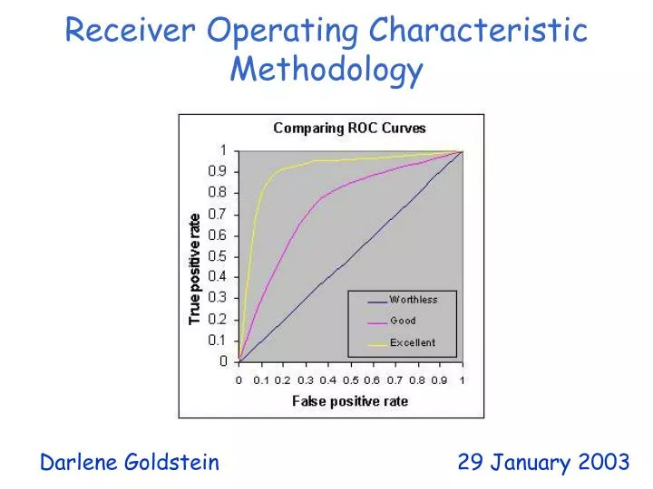
Receiver Operating Characteristic Methodology Darlene Goldstein 29 January 2003
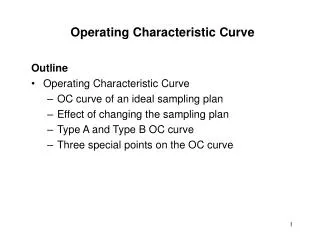
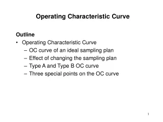
Outline • Introduction • Hypothesis testing • ROC curve • Area under the ROC curve (AUC) • Examples using ROC • Concluding remarks
Introduction to ROC curves • ROC = Receiver Operating Characteristic • Started in electronic signal detection theory (1940s - 1950s) • Has become very popular in biomedical applications, particularly radiology and imaging • Also used in machine learning applications to assess classifiers • Can be used to compare tests/procedures
ROC curves: simplest case • Consider diagnostic test for a disease • Test has 2 possible outcomes: • ‘postive’ = suggesting presence of disease • ‘negative’ • An individual can test either positive or negative for the disease • Prof. Mean...
Hypothesis testing refresher • 2 ‘competing theories’ regarding a population parameter: • NULL hypothesis H (‘straw man’) • ALTERNATIVE hypothesis A (‘claim’, or theory you wish to test) • H: NO DIFFERENCE • any observed deviation from what we expect to see is due to chance variability • A: THE DIFFERENCE IS REAL
Test statistic • Measure how far the observed data are from what is expected assuming the NULL H by computing the value of a test statistic (TS) from the data • The particular TS computed depends on the parameter • For example, to test the population mean , the TS is the sample mean (or standardized sample mean) • The NULL is rejected fi the TS falls in a user-specified ‘rejection region’
True disease state vs. Test result Test Disease
Specific Example Pts without the disease Pts with disease Test Result
Call these patients “negative” Call these patients “positive” Threshold Test Result
Call these patients “negative” Call these patients “positive” Some definitions ... True Positives Test Result without the disease with the disease
Call these patients “negative” Call these patients “positive” False Positives Test Result without the disease with the disease
Call these patients “negative” Call these patients “positive” True negatives Test Result without the disease with the disease
Call these patients “negative” Call these patients “positive” False negatives Test Result without the disease with the disease
Moving the Threshold: right ‘‘-’’ ‘‘+’’ Test Result without the disease with the disease
Moving the Threshold: left ‘‘-’’ ‘‘+’’ Test Result without the disease with the disease
ROC curve 100% True Positive Rate (sensitivity) 0% 100% 0% False Positive Rate (1-specificity)
ROC curve comparison 100% 100% True Positive Rate True Positive Rate 0% 0% 100% 100% 0% 0% False Positive Rate False Positive Rate A poor test: A good test:
ROC curve extremes 100% 100% True Positive Rate True Positive Rate 0% 0% 100% 100% 0% 0% False Positive Rate False Positive Rate Best Test: Worst test: The distributions don’t overlap at all The distributions overlap completely
‘Classical’ estimation • Binormal model: • X ~ N(0,1) in nondiseased population • X ~ N(a, 1/b) in diseased population • Then ROC(t) = (a + b-1(t)) for 0 < t < 1 • Estimate a, b by ML using readings from sets of diseased and nondiseased patients
ROC curve estimation with continuous data • Many biochemical measurements are in fact continuous, e.g. blood glucose vs. diabetes • Can also do ROC analysis for continuous (rather than binary or ordinal) data • Estimate ROC curve (and smooth) based on empirical ‘survivor’ function (1 – cdf) in diseased and nondiseased groups • Can also do regression modeling of the test result • Another approach is to model the ROC curve directlyas a function of covariates
Area under ROC curve (AUC) • Overall measure of test performance • Comparisons between two tests based on differences between (estimated) AUC • For continuous data, AUC equivalent to Mann-Whitney U-statistic (nonparametric test of difference in location between two populations)
AUC for ROC curves 100% 100% 100% 100% True Positive Rate True Positive Rate True Positive Rate True Positive Rate 0% 0% 0% 0% 100% 100% 100% 100% 0% 0% 0% 0% False Positive Rate False Positive Rate False Positive Rate False Positive Rate AUC = 100% AUC = 50% AUC = 90% AUC = 65%
Interpretation of AUC • AUC can be interpreted as the probability that the test result from a randomly chosen diseased individual is more indicative of disease than that from a randomly chosen nondiseased individual: P(Xi Xj | Di = 1, Dj = 0) • So can think of this as a nonparametric distance between disease/nondisease test results
Problems with AUC • No clinically relevant meaning • A lot of the area is coming from the range of large false positive values, no one cares what’s going on in that region (need to examine restricted regions) • The curves might cross, so that there might be a meaningful difference in performance that is not picked up by AUC
Examples using ROC analysis • Threshold selection for ‘tuning’ an already trained classifier (e.g. neural nets) • Defining signal thresholds in DNA microarrays (Bilban et al.) • Comparing test statistics for identifying differentially expressed genes in replicated microarray data (Lönnstedt and Speed) • Assessing performance of different protein prediction algorithms (Tang et al.) • Inferring protein homology (Karwath and King)
Concluding remarks – remaining challenges in ROC methodology • Inference for ROC curve when no ‘gold standard’ • Role of ROC in combining information? • Incorporating time into ROC analysis • Alternatives to ROC for describing test accuracy? • Generalization of positive/negative predictive value to continuous test? (+/-) predictive value = proportion of patients with (+/-) result who are correctly diagnosed = True/(True + False)