Download

1 / 58
580 likes | 600 Views
This course on June 11, 2019, by Dave Zhao of U of I, covers appropriate statistical methods for genomics analysis. Explore tools for complex genomic data features!

E N D
Statistics for genomics Mayo-Illinois Computational Genomics Course June 11, 2019 Dave Zhao Department of Statistics University of Illinois at Urbana-Champaign
Preparation • install.packages(c("Seurat", "glmnet", "ranger", "caret")) • Download sample GSM2818521 of GSE109158 from https://urlzs.com/7UNr6
We will illustrate how to identify the appropriate statistical method for a genomics analysis Statistical toolbox Statistical method
Classifying statistical tools Data structure Statistical task APPROPRIATE STATISTICAL METHODS
Examples from basic statistics Rosner (2015)
Distinctive features of genomic data can require specialized statistical tools to handle: • Increased complexity • Increased uncertainty • Increased scale Wu, Chen et al. (2011)
Distinctive features of genomic data can require specialized statistical tools to handle: • Increased complexity • Increased uncertainty • Increased scale New technology Wu, Chen et al. (2011)
Many variables • Distinctive features of genomic data can require specialized statistical tools to handle: • Increased complexity • Increased uncertainty • Increased scale Wu, Chen et al. (2011)
Distinctive features of genomic data can require specialized statistical tools to handle: • Increased complexity • Increased uncertainty • Increased scale Few samples Wu, Chen et al. (2011)
Distinctive features of genomic data can require specialized statistical tools to handle: • Increased complexity • Increased uncertainty • Increased scale High heterogeneity Wu, Chen et al. (2011)
We will discuss some statistical tools that are frequently used in genomics We will also discuss a general framework for organizing new tools.
Choosing the right tool for a given biological question requires creativity and experience Statistical toolbox Statistical method
There are other frameworks that are organized by biological question rather than statistical tool
To illustrate these tools, we will analyze single-cell RNA-seq data in R
Anatomy of a basic R command pandey = read.table("GSM2818521_larva_counts_matrix.txt") • Case-sensitive • Function(): performs pre-programmed calculations given inputs and options • Variable: stores values and outputs of function, name cannot contain whitespace and cannot start with a special character
Basic preprocessing of single-cell RNA-seq data using Seurat library(Seurat) s_obj = CreateSeuratObject(counts = pandey, min.cells = 3, min.features = 200) s_obj = NormalizeData(s_obj) s_obj = FindVariableFeatures(s_obj) s_obj = ScaleData(s_obj)
Where statistics appears in a standard genomic analysis workflow • Experimental design • Quality control • Preprocessing • Normalization and batch correction • Analysis • Biological interpretation Not covered today Uses statistics but is highly dependent on technology The focus of today’s discussion
Classifying statistical tools Data structure Statistical task APPROPRIATE STATISTICAL METHODS
Classifying statistical tasks Testing Supervised Plots Description Inference Estimation Tables Prediction Latent factors Unsupervised Latent groups
Classifying data structures • Can vary widely, and classification is difficult • Important factors in genomics: • Data type • Number of samples relative to number of variables
PCA > dim(pandey) [1] 24105 4365 > pandey[1:3, 1:2] larvalR2_AAACCTGAGACAGAGA.1 larvalR2_AAACCTGAGACTTTCG.1 SYN3 0 0 PTPRO 1 0 EPS8 0 0 Research question:Can the gene expression information be summarized in fewer features?
PCA Testing Supervised Plots Description Inference Estimation Tables Prediction Statistical task: calculate a (usually small) set of latent factors that captures most of the information in the dataset Data structure: can be applied to all data structures Latent factors Unsupervised Latent groups
PCA ISL Chapter 6
PCA using Seurat s_obj = RunPCA(s_obj)
Graph clustering Research question:How many cell types exist in the larval zebrafish habenula?
Graph clustering Testing Supervised Plots Description Inference Estimation Tables Prediction Statistical task: construct latent groups into which the observations fall Data structure: relatively small number of features and complicated cluster structure Latent factors Unsupervised Latent groups
Comparison to other clustering methods • Distance • Hierarchical clustering • K-means clustering vs. • Relationship • Spectral clustering • Graph clustering http://webpages.uncc.edu/jfan/itcs4122.html
Graph clustering using Seurat s_obj = FindNeighbors(s_obj, dims = 1:10) s_obj = FindClusters(s_obj, dims = 1:10, resolution = 0.1)
t-SNE plot Research question:How to visualize the different cell types?
t-SNE plot Testing Supervised Plots Description Inference Estimation Tables Prediction Statistical task: visualize observations in low dimensions Data structure: can be applied to all data structures Latent factors Unsupervised Latent groups
t-SNE plot https://en.wikipedia.org/wiki/Spring_system
t-SNE plot s_obj = RunTSNE(s_obj) DimPlot(s_obj, reduction = "tsne", label = TRUE)
Wilcoxon test Research question:Does the expression of the gene PDYN differ between clusters 5 and 6?
Wilcoxon test Testing Supervised Plots Description Inference Estimation Tables Prediction Statistical task: test whether there is an association between two variables Data structure: one variable is dichotomous Latent factors Unsupervised Latent groups
Wilcoxon test using Seurat markers = FindMarkers(s_obj, ident.1 = 5, ident.2 = 6) markers["PDYN",]
FDR control Research question:Which genes differ between clusters 5 and 6?
FDR control Testing Supervised Plots Description Inference Estimation Tables Prediction Statistical task: identify which of many hypothesis tests are truly significant Data structure: p-values are available and statistically independent Latent factors Unsupervised Latent groups
FDR control • FDR = False Discovery Rate = expected value of • Statistical methods reject the largest number of hypothesis tests while maintaining FDR , for some preset
FDR control using Seurat markers = FindMarkers(s_obj, ident.1 = 5, ident.2 = 6) head(markers) sum(markers$p_val_adj <= 0.05)
Random forest classification Research question:Given the principal components of the RNA-seq expression values of all genes from a new cell, how can we determine the cell’s type? ?
Random forest classification Testing Supervised Plots Description Inference Estimation Tables Prediction Statistical task: learn prediction rule between dependent and independent variables Data structure: one categorical dependent variable, relatively few independent variables, complicated relationship Latent factors Unsupervised Latent groups
Random forest classification Independent variables Prediction ISL Chapter 8
Random forest classification using caret and ranger library(caret) pcs = Embeddings(s_obj, reduction = "pca")[-(1:2), 1:10] class = as.factor(Idents(s_obj))[-(1:2)] dataset = data.frame(class, pcs) rf_fit = train(class ~ ., data = dataset, method = "ranger", trControl = trainControl(method = "cv", number = 3)) new_pcs = Embeddings(s_obj, reduction = "pca")[1:2, 1:10] predict(rf_fit, new_pcs) Idents(s_obj)[1:2]
Lasso Research question:If we can only measure the expression of 10 genes in a new cell, which should we measure in order to most accurately predict the cell’s type? ?