Download
1 / 12
130 likes | 181 Views
Learn how to calculate expected value and variance for discrete and continuous random variables with examples from EGR 252 Spring 2010. Understand covariance and Chebyshev's theorem. Improve your statistical knowledge.

E N D
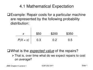
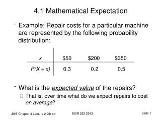
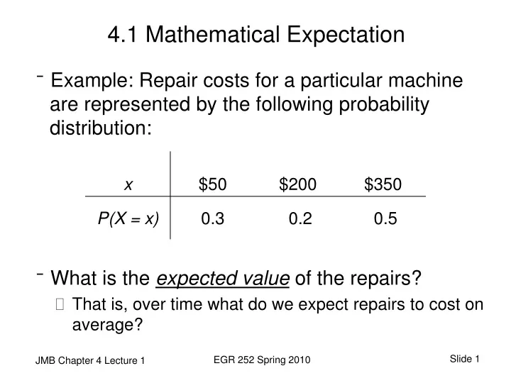
4.1 Mathematical Expectation • Example: Repair costs for a particular machine are represented by the following probability distribution: • What is the expected value of the repairs? • That is, over time what do we expect repairs to cost on average? EGR 252 Spring 2010
Expected Value – Repair Costs • μ = E(X) • μ= mean of the probability distribution • For discrete variables, μ = E(X) = ∑ x f(x) So, for our example, • E(X) = 50(0.3) + 200(0.2) + 350(0.5) = $230 EGR 252 Spring 2010
Another Example – Investment • By investing in a particular stock, a person can take a profit in a given year of $4000 with a probability of 0.3 or take a loss of $1000 with a probability of 0.7. What is the investor’s expected gain on the stock? X $4000 -$1000 P(X) 0.3 0.7 E(X) = $4000 (0.3) -$1000(0.7) = $500 EGR 252 Spring 2010
Expected Value - Continuous Variables • For continuous variables, μ = E(X) = E(X) = ∫ x f(x) dx • Vacuum cleaner example: problem 7 pg. 88 x, 0 < x < 1 f(x) = 2-x, 1 ≤ x < 2 0, elsewhere (in hundreds of hours.) { = 1 * 100 = 100.0 hours of operation annually, on average EGR 252 Spring 2010
Functions of Random Variables • Ex 4.4. pg. 111: Probability of X, the number of cars passing through a car wash in one hour on a sunny Friday afternoon, is given by • Let g(X) = 2X -1 represent the amount of money paid to the attendant by the manager. What can the attendant expect to earn during this hour on any given sunny Friday afternoon? E[g(X)] =Σg(x) f(x) = Σ (2X-1) f(x) = (2*4-1)(1/12) +(2*5-1)(1/12) …+(2*9-1)(1/6) = $12.67 EGR 252 Spring 2010
4.2 Variance of a Random Variable • Recall our example: Repair costs for a particular machine are represented by the following probability distribution: • What is the variance of the repair cost? • That is, how might we define the spread of costs? EGR 252 Spring 2010
Variance – Discrete Variables • For discrete variables, • σ2 = E [(X - μ)2] = ∑ (x - μ)2 f(x) = E (X2) - μ2 • Recall, for our example, μ = E(X) = $230 • Preferred method of calculation: • σ2 = [E(X2)] – μ2 = 502 (0.3) + 2002 (0.2) + 3502 (0.5) – 2302 = $17,100 • Alternate method of calculation: • σ2 = E(X- μ)2 f(x) = (50-230)2 (0.3) + (200-230)2 (0.2) + (350-230)2 (0.5) = $17,100 EGR 252 Spring 2010
Variance - Investment Example • By investing in a particular stock, a person can take a profit in a given year of $4000 with a probability of 0.3 or take a loss of $1000 with a probability of 0.7. What are the variance and standard deviation of the investor’s gain on the stock? • E(X) = $4000 (0.3) -$1000 (0.7) = $500 • σ2 = [∑(x2 f(x))] – μ2 = (4000)2(0.3) + (-1000)2(0.7) – 5002 = $5,250,000 • σ = $2291.29 EGR 252 Spring 2010
Variance of Continuous Variables • For continuous variables, σ2 = E [(X - μ)2] =[∫ x2 f(x) dx] – μ2 • Recall our vacuum cleaner example pr. 7 pg. 88 x, 0 < x < 1 f(x) = 2-x, 1 ≤ x < 2 0, elsewhere (in hundreds of hours of operation.) • What is the variance of X? The variable is continuous, therefore we will need to evaluate the integral. { EGR 252 Spring 2010
Variance Calculations for Continuous Variables • (Preferred calculation) • What is the standard deviation? • σ = 0.4082 hours EGR 252 Spring 2010
Covariance • A measure of the nature of the association between two variables • Describes a potential linear relationship • Positive relationship • Large values of X result in large values of Y • Negative relationship • Large values of X result in small values of Y • “Manual” calculations are based on the joint probability distributions • Statistical software is more often used to calculate the correlation coefficient EGR 252 Spring 2010
What if the distribution is unknown? • Chebyshev’s theorem: The probability that any random variable X will assume a value within k standard deviations of the mean is at least 1 – 1/k2. That is, P(μ – kσ < X < μ + kσ) ≥ 1 – 1/k2 • “Distribution-free” theorem – results are weak • If we believe we “know” the distribution, we do not use Chebyshev’s theorem to characterize variability EGR 252 Spring 2010