Download
1 / 20
220 likes | 559 Views
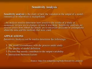
Sensitivity Analysis. Introduction to Sensitivity Analysis Graphical Sensitivity Analysis Sensitivity Analysis: Computer Solution Simultaneous Changes. Introduction to Sensitivity Analysis.

E N D
Sensitivity Analysis • Introduction to Sensitivity Analysis • Graphical Sensitivity Analysis • Sensitivity Analysis: Computer Solution • Simultaneous Changes
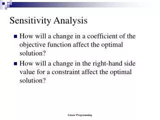
Introduction to Sensitivity Analysis • Sensitivity analysis (or post-optimality analysis) is used to determine how the optimal solution is affected by changes, within specified ranges, in: • the objective function coefficients • the right-hand side (RHS) values • Sensitivity analysis is important to a manager who must operate in a dynamic environment with imprecise estimates of the coefficients. • Sensitivity analysis allows a manager to ask certain what-if questions about the problem.
Example 1 • LP Formulation Max 5x1 + 7x2 s.t. x1< 6 2x1 + 3x2< 19 x1 + x2< 8 x1, x2> 0
Example 1 • Graphical Solution x2 x1 + x2< 8 8 7 6 5 4 3 2 1 Max 5x1 + 7x2 x1< 6 Optimal Solution: x1 = 5, x2 = 3 2x1 + 3x2< 19 x1 1 2 3 4 5 6 7 8 9 10
Objective Function Coefficients • Let us consider how changes in the objective function coefficients might affect the optimal solution. • The range of optimality for each coefficient provides the range of values over which the current solution will remain optimal. • Managers should focus on those objective coefficients that have a narrow range of optimality and coefficients near the endpoints of the range.
Example 1 • Changing Slope of Objective Function x2 Coincides with x1 + x2< 8 constraint line 8 7 6 5 4 3 2 1 Objective function line for 5x1 + 7x2 5 Coincides with 2x1 + 3x2< 19 constraint line Feasible Region 4 3 1 2 x1 1 2 3 4 5 6 7 8 9 10
Range of Optimality • Graphically, the limits of a range of optimality are found by changing the slope of the objective function line within the limits of the slopes of the binding constraint lines. • Slope of an objective function line, Max c1x1 + c2x2, is -c1/c2, and the slope of a constraint, a1x1 + a2x2 = b, is -a1/a2.
Example 1 • Range of Optimality for c1 The slope of the objective function line is -c1/c2. The slope of the first binding constraint, x1 + x2 = 8, is -1 and the slope of the second binding constraint, x1 + 3x2 = 19, is -2/3. Find the range of values for c1 (with c2 staying 7) such that the objective function line slope lies between that of the two binding constraints: -1 < -c1/7 < -2/3 Multiplying through by -7 (and reversing the inequalities): 14/3 <c1< 7
Example 1 • Range of Optimality for c2 Find the range of values for c2 ( with c1 staying 5) such that the objective function line slope lies between that of the two binding constraints: -1 < -5/c2< -2/3 Multiplying by -1: 1 > 5/c2> 2/3 Inverting, 1 <c2/5 < 3/2 Multiplying by 5: 5 <c2< 15/2
Sensitivity Analysis: Computer Solution Software packages such as The Management Scientist and Microsoft Excel provide the following LP information: • Information about the objective function: • its optimal value • coefficient ranges (ranges of optimality) • Information about the decision variables: • their optimal values • their reduced costs • Information about the constraints: • the amount of slack or surplus • the dual prices • right-hand side ranges (ranges of feasibility)
Example 1 • Range of Optimality for c1 and c2 Adjustable Cells Final Reduced Objective Allowable Allowable Cell Name Value Cost Coefficient Increase Decrease $B$8 X1 5.0 0.0 5 2 0.33333333 $C$8 X2 3.0 0.0 7 0.5 2 Constraints Final Shadow Constraint Allowable Allowable Cell Name Value Price R.H. Side Increase Decrease $B$13 #1 5 0 6 1E+30 1 $B$14 #2 19 2 19 5 1 $B$15 #3 8 1 8 0.33333333 1.66666667
Right-Hand Sides • Let us consider how a change in the right-hand side for a constraint might affect the feasible region and perhaps cause a change in the optimal solution. • The improvement in the value of the optimal solution per unit increase in the right-hand side is called the dual price. • The range of feasibility is the range over which the dual price is applicable. • As the RHS increases, other constraints will become binding and limit the change in the value of the objective function.
Dual Price • Graphically, a dual price is determined by adding +1 to the right hand side value in question and then resolving for the optimal solution in terms of the same two binding constraints. • The dual price is equal to the difference in the values of the objective functions between the new and original problems. • The dual price for a nonbinding constraint is 0. • A negative dual price indicates that the objective function will not improve if the RHS is increased.
Relevant Cost and Sunk Cost • A resource cost is a relevant cost if the amount paid for it is dependent upon the amount of the resource used by the decision variables. • Relevant costs are reflected in the objective function coefficients. • A resource cost is a sunk cost if it must be paid regardless of the amount of the resource actually used by the decision variables. • Sunk resource costs are not reflected in the objective function coefficients.
Cautionary Note onthe Interpretation of Dual Prices • Resource cost is sunk The dual price is the maximum amount you should be willing to pay for one additional unit of the resource. • Resource cost is relevant The dual price is the maximum premium over the normal cost that you should be willing to pay for one unit of the resource.
Example 1 • Dual Prices Constraint 1: Since x1< 6 is not a binding constraint, its dual price is 0. Constraint 2: Change the RHS value of the second constraint to 20 and resolve for the optimal point determined by the last two constraints: 2x1 + 3x2 = 20 and x1 + x2 = 8. The solution is x1 = 4, x2 = 4, z = 48. Hence, the dual price = znew - zold = 48 - 46 = 2.
Example 1 • Dual Prices Constraint 3: Change the RHS value of the third constraint to 9 and resolve for the optimal point determined by the last two constraints: 2x1 + 3x2 = 19 and x1 + x2 = 9. The solution is: x1 = 8, x2 = 1, z = 47. The dual price is znew - zold = 47 - 46 = 1.
Example 1 • Dual Prices Adjustable Cells Final Reduced Objective Allowable Allowable Cell Name Value Cost Coefficient Increase Decrease $B$8 X1 5.0 0.0 5 2 0.33333333 $C$8 X2 3.0 0.0 7 0.5 2 Constraints Final Shadow Constraint Allowable Allowable Cell Name Value Price R.H. Side Increase Decrease $B$13 #1 5 0 6 1E+30 1 $B$14 #2 19 2 19 5 1 $B$15 #3 8 1 8 0.33333333 1.66666667
Range of Feasibility • The range of feasibility for a change in the right hand side value is the range of values for this coefficient in which the original dual price remains constant. • Graphically, the range of feasibility is determined by finding the values of a right hand side coefficient such that the same two lines that determined the original optimal solution continue to determine the optimal solution for the problem.
Example 1 • Range of Feasibility Adjustable Cells Final Reduced Objective Allowable Allowable Cell Name Value Cost Coefficient Increase Decrease $B$8 X1 5.0 0.0 5 2 0.33333333 $C$8 X2 3.0 0.0 7 0.5 2 Constraints Final Shadow Constraint Allowable Allowable Cell Name Value Price R.H. Side Increase Decrease $B$13 #1 5 0 6 1E+30 1 $B$14 #2 19 2 19 5 1 $B$15 #3 8 1 8 0.33333333 1.66666667