Download
1 / 33
330 likes | 506 Views
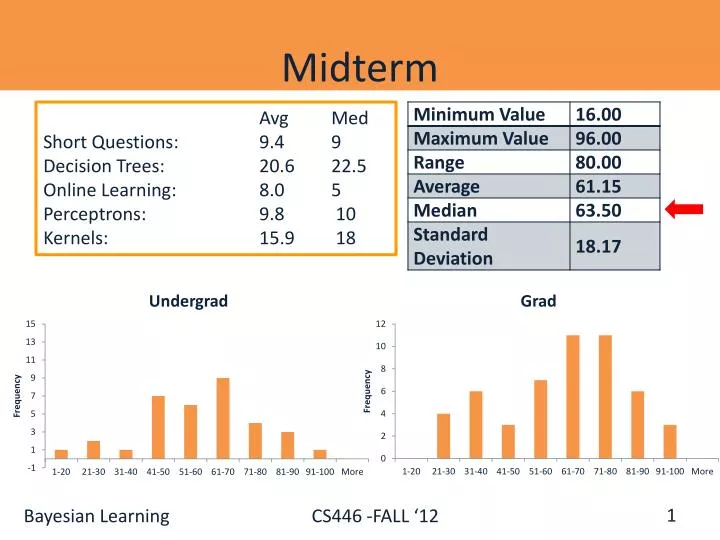
Midterm. Avg Med Short Questions: 9.4 9 Decision Trees: 20.6 22.5 Online Learning: 8.0 5 Perceptrons : 9.8 10 Kernels: 15.9 18. Recap: Error Driven Learning . Consider a distribution D over space X Y

E N D
Midterm Avg Med Short Questions: 9.4 9 Decision Trees: 20.6 22.5 Online Learning: 8.0 5 Perceptrons: 9.8 10 Kernels: 15.9 18
Recap: Error Driven Learning Consider a distribution D over space XY X - the instance space; Y - set of labels. (e.g. +/-1) Can think about the data generation process as governed by D(x), and the labeling process as governed by D(y|x), such that D(x,y)=D(x) D(y|x) This can be used to model both the case where labels are generated by a function y=f(x), as well as noisy cases and probabilistic generation of the label. If the distribution D is known, there is no learning. We can simply predict y = argmaxy D(y|x) If we are looking for a hypothesis, we can simply find the one that minimizes the probability of mislabeling: h = argminh E(x,y)~D [[h(x) y]]
Recap: Error Driven Learning (2) Inductive learning comes into play when the distribution is not known. Then, there are two basic approaches to take. Discriminative (direct) learning and Bayesian Learning (Generative)
1: Direct Learning Model the problem of text correction as a problem of learning from examples. Goal: learn directly how to make predictions. PARADIGM Look at many (postive/negative) examples. Discover some regularities in the data. Use these to construct a prediction policy. A policy (a function, a predictor) needs to be specific. [it/in] rule: if the occurs after the target in Assumptions comes in the form of a hypothesis class.
Direct Learning (2) Consider a distribution D over space XY X - the instance space; Y - set of labels. (e.g. +/-1) Given a sample {(x,y)}1m,, and a loss function L(x,y) Find hH that minimizes i=1,mD(xi,yi)L(h(xi),yi) + Reg L can be: L(h(x),y)=1, h(x)y, o/w L(h(x),y) = 0 (0-1 loss) L(h(x),y)=(h(x)-y)2 , (L2 ) L(h(x),y)= max{0,1-y h(x)} (hinge loss) L(h(x),y)= exp{- yh(x)} (exponential loss) Find an algorithm that minimizes average losson the observed data. Then, we know that things will be okay (as a function of H).
2: Generative Model • Model the problem of text correction as that of generating correct sentences. • Goal: learn a model of the language; use it to predict. PARADIGM • Learn a probability distribution over all sentences • In practice: make assumptions on the distribution’s type • Use it to estimate which sentence is more likely. • Pr(I saw the girl it the park) <> Pr(I saw the girl in the park) • In practice: a decision policy depends on the assumptions
Probabilistic Learning • There are actually two different notions. • Learning probabilistic concepts • The learned concept is a function c:X[0,1] • c(x) may be interpreted as the probability that the label 1 is assigned to x • The learning theory that we have studied before is applicable (with some extensions). • Bayesian Learning: Use of a probabilistic criterion in selecting a hypothesis • The hypothesis can be deterministic, a Boolean function. • It’s not the hypothesis – it’s the process.
Basics of Bayesian Learning • Goal: find the best hypothesis from some space H of hypotheses, given the observed data D. • Define best to be: most probable hypothesis in H • In order to do that, we need to assume a probability distribution over the class H. • In addition, we need to know something about the relation between the data observed and the hypotheses (E.g., a coin problem.) • As we will see, we will be Bayesian about other things, e.g., the parameters of the model
Basics of Bayesian Learning P(h) - the prior probability of a hypothesis h Reflects background knowledge; before data is observed. If no information - uniform distribution. P(D) - The probability that this sample of the Data is observed. (No knowledge of the hypothesis) P(D|h): The probability of observing the sample D, given that hypothesis h is the target P(h|D): The posterior probability of h. The probability that h is the target, given that D has been observed.
Bayes Theorem P(h|D) increases with P(h) and with P(D|h) P(h|D) decreases with P(D)
Basic Probability • Product Rule: P(A,B) = P(A|B)P(B) = P(B|A)P(A) • If A and B are independent: • P(A,B) = P(A)P(B); P(A|B)= P(A), P(A|B,C)=P(A|C) • Sum Rule:P(AB) = P(A)+P(B)-P(A,B) • Bayes Rule: P(A|B) = P(B|A) P(A)/P(B) • Total Probability: • If events A1, A2,…An are mutually exclusive: AiÅAj = Á, iAi = 1 • P(B) = P(B , Ai) = iP(B|Ai) P(Ai) • Total Conditional Probability: • If events A1, A2,…Anare mutually exclusive: AiÅAj= Á, iAi= 1 • P(B|C) = P(B , Ai|C) = iP(B|Ai,C) P(Ai|C)
Learning Scenario P(h|D) = P(D|h) P(h)/P(D) The learner considers a set of candidate hypotheses H (models), and attempts to find the most probableone h H, given the observed data. Such maximally probable hypothesis is called maximum a posteriori hypothesis (MAP); Bayes theorem is used to compute it: hMAP = argmaxh2 H P(h|D) = argmaxh2 H P(D|h) P(h)/P(D) = argmaxh2 H P(D|h) P(h)
Learning Scenario (2) hMAP = argmaxh2 H P(h|D) = argmaxh2 H P(D|h) P(h) We may assume that a priori, hypotheses are equally probable: P(hi) = P(hj) 8hi, hj2 H We get the Maximum Likelihood hypothesis: hML = argmaxh2 H P(D|h) Here we just look for the hypothesis that best explains the data
Examples • hMAP = argmaxh2 H P(h|D) = argmaxh2 H P(D|h) P(h) • A given coin is either fair or has a 60% bias in favor of Head. • Decide what is the bias of the coin [This is a learning problem!] • Two hypotheses: h1: P(H)=0.5; h2: P(H)=0.6 • Prior: P(h): P(h1)=0.75 P(h2 )=0.25 • Now we need Data. 1stExperiment: coin toss is H. • P(D|h): P(D|h1)=0.5 ; P(D|h2) =0.6 • P(D): P(D)=P(D|h1)P(h1) + P(D|h2)P(h2 ) = 0.5 0.75 + 0.6 0.25 = 0.525 • P(h|D): P(h1|D) = P(D|h1)P(h1)/P(D) = 0.50.75/0.525 = 0.714 P(h2|D) = P(D|h2)P(h2)/P(D) = 0.60.25/0.525 = 0.286
Examples(2) • hMAP = argmaxh2 H P(h|D) = argmaxh2 H P(D|h) P(h) • A given coin is either fair or has a 60% bias in favor of Head. • Decide what is the bias of the coin [This is a learning problem!] • Two hypotheses: h1: P(H)=0.5; h2: P(H)=0.6 • Prior: P(h): P(h1)=0.75 P(h2 )=0.25 • After 1st coin toss is H we still think that the coin is more likely to be fair • If we were to use Maximum Likelihood approach (i.e., assume equal priors) we would think otherwise. The data supports the biased coin better. • Try: 100 coin tosses; 70 heads. • You will believe that the coins is biased.
Examples(2) • hMAP = argmaxh2 H P(h|D) = argmaxh2 H P(D|h) P(h) • A given coin is either fair or has a 60% bias in favor of Head. • Decide what is the bias of the coin [This is a learning problem!] • Two hypotheses: h1: P(H)=0.5; h2: P(H)=0.6 • Prior: P(h): P(h1)=0.75 P(h2 )=0.25 • Case of 100 coin tosses; 70 heads. P(D) = P(D|h1) P(h1) + P(D|h2) P(h2) = = 0.5100¢ 0.75 + 0.670¢0.430¢ 0.25 = = 7.9 ¢10-31¢ 0.75 + 3.4 ¢10-28¢ 0.25 0.0057 = P(h1|D) = P(D|h1) P(h1)/P(D) <<P(D|h2) P(h2) /P(D) = P(h2|D) =0.9943
Example: Learning a Concept Class Assume that we are given a concept class C. Given a collection of examples (x,f(x)), For f C, we try to identify h that is consistent with f on the training data. We showed that it will do well in the future. What will the Bayesian approach tell us ?
{ Learning a Concept Class P(h): the prior probability of a hypothesis h: p(h) = 1/|H| for all h in H P(D|h): Let d=(x,l) be the observed labeled example P((x,l)|h)= 1, if h(x)=l; P((x,l)|h) = 0 (if h(x)<>l) (same for a set D of examples: possible if the examples are labeled correctly) P(D): For a set of D examples: where HCON is the set of hypotheses in H which are consistent with the sample D P(h|D): via Bayes rule
Example: A Model of Language Consider Strings: AABBC & ABBBA You observe a string; use it to learn the language model. E.g., S= AABBABC; Compute P(A) Model 1: There are 5 characters, A, B, C, D, E, and space At any point can generate any of them, according to: P(A)= p1; P(B) =p2; P(C) =p3; P(D)= p4; P(E)= p5 P(SP)= p6 i pi = 1 E.g., P(A)= 0.3; P(B) =0.1; P(C) =0.2; P(D)= 0.2; P(E)= 0.1 P(SP)=0.1 We assume a generative model of independent characters: P(U) = P(x1, x2,…, xk)= i=1,k P(xi| xi+1, xi+2,…, xk)= i=1,k P(xi) The parameters of the model are the character generation probabilities (Unigram). Goal: to determine which of two strings U, V is more likely. The Bayesian way: compute the probability of each string, and decide which is more likely. Learning here is: learning the parameters of a known model family How?
1. The model we assumed is binomial. You could assume a different model! Next we will consider other models and see how to learn their parameters. Maximum Likelihood Estimate 2. In practice, smoothing is advisable - equivalent to assuming a different model. Assume that you toss a (p,1-p) coin m times and get k Heads, m-k Tails. What is p? If p is the probability of Head, the probability of the data observed is: P(D|p) = pk(1-p)m-k The log Likelihood: L(p) = log P(D|p) = k log(p) + (m-k)log(1-p) To maximize, set the derivative w.r.t. p equal to 0: dL(p)/dp = k/p – (m-k)/(1-p) Solving this for p, gives: p=k/m
Probability Distributions • Bernoulli Distribution: • Random Variable X takes values {0, 1} s.t P(X=1) = p = 1 – P(X=0) • Binomial Distribution: • Random Variable X takes values {1, 2,…, n} representing the number of successes (X=1) in n Bernoulli trials. • P(X=k) = f(n, p, k) = Cnkpk (1-p)n-k • Note that if X ~ Binom(n, p) and Y ~ Bernulli (p), X = i=1,n Y TexPoint fonts used in EMF. Read the TexPoint manual before you delete this box.: AAAAA
Probability Distributions(2) • Categorical Distribution: • Random Variable X takes on values in {1,2,…k} s.t P(X=i) = pi and 1kpi = 1 • Multinomial Distribution: is to Categorical what Binomial is to Bernoulli • Let the random variables Xi (i=1, 2,…, k) indicates the number of times outcome i was observed over the n trials. • The vector X = (X1, ..., Xk) follows a multinomial distribution (n,p) where p = (p1, ..., pk) and 1kpi = 1 • f(x1, x2,…xk, n, p) = P(X1= x1, … Xk = xk) = TexPoint fonts used in EMF. Read the TexPoint manual before you delete this box.: AAAAA
A Multinomial Bag of Words • We are given a collection of documents written in a three word language {a, b, c}. All the documents have exactly n words (each word can be either a, b or c). • We are given a labeled document collection {D1, D2 ... , Dm}. The label yiof document Diis 1 or 0, indicating whether Diis “good” or “bad”. • This model uses the multinominal distributions. That is, ai(bi,ci, resp.) is the number of times word a (b, c, resp.) appears in document Di. • Therefore: ai+ bi+ ci= |Di| = n. • In this model, we have: P(Di|y = 1) =n!/(ai! bi! ci!) ®1ai¯1bi°1ci where ®1 (¯1, °1resp.) is the probability that a (b , c) appears in a “good” document. • Similarly, P(Di|y= 0) =n!/(ai! bi! ci!) ®0ai¯0bi°0ci • Note that: ®0+¯0+°0=®1+¯1+°1 =1 TexPoint fonts used in EMF. Read the TexPoint manual before you delete this box.: AAAAA
A Multinomial Bag of Words (2) • We are given a collection of documents written in a three word language {a, b, c}. All the documents have exactly n words (each word can be either a, b or c). • We are given a labeled document collection {D1, D2 ... , Dm}. The label yiof document Diis 1 or 0, indicating whether Diis “good” or “bad”. • The classification problem: given a document D, determine if it is good or bad; that is, determine P(y|D). • This can be determined via Bayes rule: P(y|D) = P(D|y) P(y)/P(D) • But, we need to know the parameters of the model to compute that. TexPoint fonts used in EMF. Read the TexPoint manual before you delete this box.: AAAAA
Notice that this is an important trick to write down the joint probability without knowing what the outcome of the experiment is. The ith expression evaluates to p(Di , yi) (Could be written with sum of multiplicativeyi but less convenient) A Multinomial Bag of Words (3) • How do we estimate the parameters? • We derive the most likely value of the parameters defined above by maximizing the log likelihood of the observed data. • PD = PiP(yi , Di ) = PiP(Di |yi ) P(yi) = • We denote by ´the probability that an example is “good” (yi=1; otherwise yi=0). Then: • Pi P(y, Di ) = Pi [(´n!/(ai! bi! ci!) ®1ai¯1bi°1ci)yi¢((1 - ´) n!/(ai! bi! ci!) ®0ai¯0bi°0ci )1-yi] • We want to maximize it with respect to each of the parameters. We first compute log (PD) and then differentiate: • log(PD) =iyi [ log(´) + C + ai log(®1) + bi log(¯1) + ci log(°1) + (1- yi) [log(1-´) + C’ + ailog(®0) + bilog(¯0) + cilog(°0) ] • dlogPD/d ´ = i [yi /´ - (1-yi)/(1-´)] = 0 i (yi - ´) = 0 ´ = iyi /m • The same can be done for the other 6 parameters. However, notice that they are not independent: ®0+¯0+°0=®1+¯1+°1 =1 and also ai+ bi+ ci= |Di| = n. Labeled data, assuming that the examples are independent TexPoint fonts used in EMF. Read the TexPoint manual before you delete this box.: AAAAA
0.8 0.8 0.5 0.5 P(B)=0.5 P(I)=0.5 0.2 0.2 B I P(x|B) P(x|I) 0.5 0.5 0.2 0.5 0.5 0.5 B I I I B 0.5 0.25 0.25 0.25 0.25 0.4 a a c d d Other Examples (HMMs) • We can do the same exercise we did before. • Data: {(x1 ,x2,…xm ,s1 ,s2,…sm)}1n • Find the most likely parameters of the model: • P(xi |si), P(si+1 |si), p(s1) (easier than previous case) • Given an unlabeled example • x = (x1, x2,…xm) • use Bayes rule to predict the label l=(s1, s2,…sm): • l* = argmaxl P(l|x) = argmaxl P(x|l) P(l)/P(x) • The only issue is computational: there are 2m possible values of l • Consider data over 5 characters, x=a, b, c, d, e, and 2 states s=B, I • We generate characters according to: • Initial state prob: p(B)= 0.5; p(I)=0.5 • State transition prob: • p(BB)=0.8 p(BI)=0.2 • p(IB)=0.5 p(II)=0.5 • Output prob: • p(a|B) = 0.25,p(b|B)=0.10, p(c|B)=0.10 • … • p(a|I) = 0.25,… • Can follow the generation process to get the observed sequence.
Bayes Optimal Classifier How should we use the general formalism? What should H be? H can be a collection of functions. Given the training data, choose an optimal function. Then, given new data, evaluate the selected function on it. H can be a collection of possible predictions. Given the data, try to directly choose the optimal prediction. Could be different!
Bayes Optimal Classifier The first formalism suggests to learn a good hypothesis and use it. (Language modeling, grammar learning, etc. are here) The second one suggests to directly choose a decision.[accept or except]: This is the issue of “thresholding” vs. entertaining all options until the last minute. (Computational Issues)
Bayes Optimal Classifier: Example • Assume a space of 3 hypotheses: • P(h1|D) = 0.4; P(h2|D) = 0.3; P(h3|D) = 0.3 hMAP = h1 • Given a new instance, assume that • h1(x) = 1 h2(x) = 0 h3(x) = 0 • In this case, • P(f(x) =1 ) = 0.4 ; P(f(x) = 0) = 0.6 but hMAP (x) =1 • We want to determine the most probable classification by combining the prediction of all hypotheses, weighted by their posterior probabilities
Bayes Optimal Classifier: Example(2) • Let V be a set of possible classifications • Bayes Optimal Classification: • In the example: • and the optimal prediction is indeed 0. • The key example of using a “Bayes optimal Classifier” is that of the naïve Bayes algorithm.
Justification: Bayesian Approach The Bayes optimal function is fB(x) = argmaxyD(x; y) That is, given input x, return the most likely label It can be shown thatfBhas the lowest possible value forErr(f) Caveat: we can never construct this function: it is a function ofD, which is unknown. But, it is a useful theoretical construct, and drives attempts to make assumptions onD
Maximum-Likelihood Estimates • We attempt to model the underlying distribution D(x, y) or D(y | x) • To do that, we assume a model P(x, y | ) or P(y | x , ), where is the set of parameters of the model • Example: Probabilistic Language Model (Markov Model): • We assume a model of language generation. Therefore, P(x, y | ) was written as a function symbol & state probabilities(the parameters). • We typically look at the log-likelihood • Given training samples (xi; yi), maximize the log-likelihood • L() = i log P (xi; yi | ) or L() = i log P (yi | xi , ))
Justification: Bayesian Approach Are we done? We provided also Learning Theory explanations for why these algorithms work. Assumption: Our selection of the model is good; there is some parameter setting * such that the true distribution is really represented by our model D(x, y) = P(x, y | *) Define the maximum-likelihood estimates: ML = argmaxL() As the training sample size goes to , then P(x, y | ML) converges to D(x, y) Given the assumption above, and the availability of enough data argmaxyP(x, y | ML) converges to the Bayes-optimal function fB(x) = argmaxyD(x; y)