Download
1 / 21
230 likes | 443 Views
Ch 7.9: Nonhomogeneous Linear Systems. The general theory of a nonhomogeneous system of equations parallels that of a single n th order linear equation. This system can be written as x ' = P ( t ) x + g ( t ), where. General Solution.

E N D
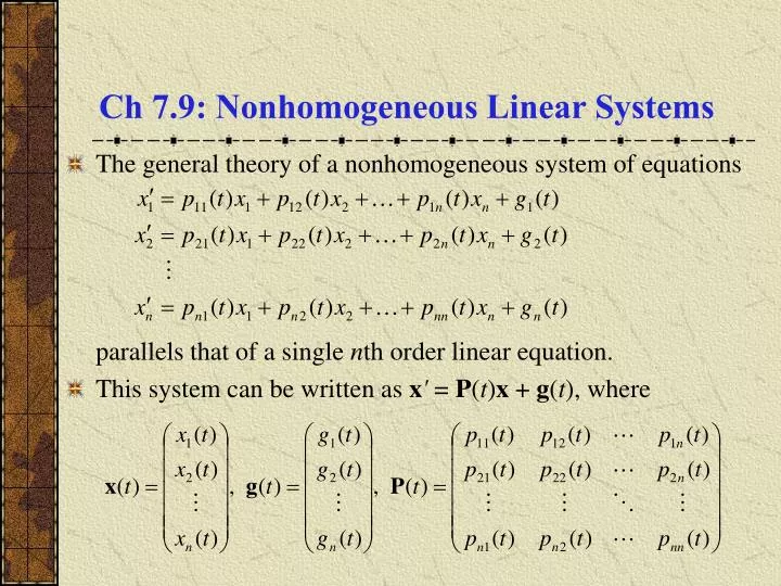
Ch 7.9: Nonhomogeneous Linear Systems • The general theory of a nonhomogeneous system of equations parallels that of a single nth order linear equation. • This system can be written as x' = P(t)x + g(t), where
General Solution • The general solution of x' = P(t)x + g(t) on I: < t < has the form where is the general solution of the homogeneous system x' = P(t)x and v(t) is a particular solution of the nonhomogeneous system x' = P(t)x + g(t).
Diagonalization • Suppose x' = Ax + g(t), where A is an n x n diagonalizable constant matrix. • Let T be the nonsingular transform matrix whose columns are the eigenvectors of A, and D the diagonal matrix whose diagonal entries are the corresponding eigenvalues of A. • Suppose x satisfies x' = Ax+g(t),, let y be defined by x = Ty. • Substituting x = Ty into x' = Ax + g(t), we obtain Ty'= ATy + g(t). or y'= T-1ATy + T-1g(t) or y'= Dy + h(t), where h(t) = T-1g(t). • Note that if we can solve diagonal system y'= Dy + h(t) for y, then x = Ty is a solution to the original system.
Solving Diagonal System • Nowy'= Dy + h(t) is a diagonal system of the form where r1,…, rn are the eigenvalues of A. • Thus y'= Dy + h(t) is an uncoupled system of n linear first order equations in the unknowns yk(t), which can be isolated and solved separately, using methods of Section 2.1:
Solving Original System • The solution y toy'= Dy + h(t) has components • For this solution vector y, the solution to the original system x' = Ax + g(t) is then x = Ty. • Recall that T is the nonsingular transform matrix whose columns are the eigenvectors of A. • Thus, when multiplied by T, the second term on right side of yk produces general solution of homogeneous equation, while the integral term of yk produces a particular solution of nonhomogeneous system.
Example 1: General Solution of Homogeneous Case (1 of 5) • Consider the nonhomogeneous system x' = Ax + g below. • Note: A is a Hermitian matrix, since it is real and symmetric. • The eigenvalues of A are r1 = -3 and r2= -1, with corresponding eigenvectors • The general solution of the homogeneous system is then
Example 1: Transformation Matrix (2 of 5) • Consider next the transformation matrix T of eigenvectors. Using a Section 7.7 comment, and A Hermitian, we have T-1 = T* = TT, provided we normalize (1)and (2) so that ((1), (1)) = 1 and ((2), (2)) = 1. Thus normalize as follows: • Then for this choice of eigenvectors,
Example 1: Diagonal System and its Solution (3 of 5) • Under the transformation x = Ty, we obtain the diagonal system y'= Dy + T-1g(t): • Then, using methods of Section 2.1,
Example 1: Transform Back to Original System (4 of 5) • We next use the transformation x = Ty to obtain the solution to the original system x'= Ax + g(t):
Example 1: Solution of Original System (5 of 5) • Simplifying further, the solution x can be written as • Note that the first two terms on right side form the general solution to homogeneous system, while the remaining terms are a particular solution to nonhomogeneous system.
Undetermined Coefficients • A second way of solving x' = P(t)x + g(t) is the method of undetermined coefficients. Assume P is a constant matrix, and that the components of g are polynomial, exponential or sinusoidal functions, or sums or products of these. • The procedure for choosing the form of solution is usually directly analogous to that given in Section 3.6. • The main difference arises when g(t) has the form uet,where is a simple eigenvalue of P. In this case, g(t) matches solution form of homogeneous system x' = P(t)x, and as a result, it is necessary to take nonhomogeneous solution to be of the form atet + bet. This form differs from the Section 3.6 analog, atet.
Example 2: Undetermined Coefficients (1 of 5) • Consider again the nonhomogeneous system x' = Ax + g: • Assume a particular solution of the form where the vector coefficients a, b, c, d are to be determined. • Since r = -1 is an eigenvalue of A, it is necessary to include both ate-t and be-t, as mentioned on the previous slide.
Example 2: Matrix Equations for Coefficients (2 of 5) • Substituting in for x in our nonhomogeneous system x'= Ax + g, we obtain • Equating coefficients, we conclude that
Example 2: Solving Matrix Equation for a(3 of 5) • Our matrix equations for the coefficients are: • From the first equation, we see that a is an eigenvector of A corresponding to eigenvalue r = -1, and hence has the form • We will see on the next slide that = 1, and hence
Example 2: Solving Matrix Equation for b(4 of 5) • Our matrix equations for the coefficients are: • Substituting aT = (,) into second equation, • Thus = 1, and solving for b, we obtain
Example 2: Particular Solution (5 of 5) • Our matrix equations for the coefficients are: • Solving third equation for c, and then fourth equation for d, it is straightforward to obtain cT = (1, 2), dT = (-4/3, -5/3). • Thus our particular solution of x' = Ax + g is • Comparing this to the result obtained in Example 1, we see that both particular solutions would be the same if we had chosen k = ½ for b on previous slide, instead of k = 0.
Variation of Parameters: Preliminaries • A more general way of solving x' = P(t)x + g(t) is the method of variation of parameters. • Assume P(t) and g(t) are continuous on < t < , and let (t) be a fundamental matrix for the homogeneous system. • Recall that the columns of are linearly independent solutions of x' = P(t)x, and hence (t) is invertible on the interval < t < , and also '(t) = P(t)(t). • Next, recall that the solution of the homogeneous system can be expressed as x = (t)c. • Analogous to Section 3.7, assume the particular solution of the nonhomogeneous system has the form x = (t)u(t), where u(t) is a vector to be found.
Variation of Parameters: Solution • We assume a particular solution of the form x = (t)u(t). • Substituting this into x' = P(t)x + g(t), we obtain '(t)u(t) + (t)u'(t) = P(t)(t)u(t) + g(t) • Since '(t) = P(t)(t), the above equation simplifies to u'(t) = -1(t)g(t) • Thus where the vector c is an arbitrary constant of integration. • The general solution to x' = P(t)x + g(t) is therefore
Variation of Parameters: Initial Value Problem • For an initial value problem x'= P(t)x + g(t), x(t0) = x(0), the general solution to x' = P(t)x + g(t) is • In practice, it may be easier to row reduce matrices and solve necessary equations than to compute -1(t) and substitute into equations.
Summary (1 of 2) • The method of undetermined coefficients requires no integration but is limited in scope and may involve several sets of algebraic equations. • Diagonalization requires finding inverse of transformation matrix and solving uncoupled first order linear equations. When coefficient matrix is Hermitian, the inverse of transformation matrix can be found without calculation, which is very helpful for large systems.
Summary (2 of 2) • Variation of parameters is the most general method, but it involves solving linear algebraic equations with variable coefficients, integration, and matrix multiplication, and hence may be the most computationally complicated method. • For many small systems with constant coefficients, all of these methods work well, and there may be little reason to select one over another.